17 Introduction to Hypothesis Testing

What is Hypothesis Testing?

Hypothesis testing is a big part of what we would actually consider testing for inferential statistics. It’s a procedure and set of rules that allow us to move from descriptive statistics to make inferences about a population based on sample data. It is a statistical method that uses sample data to evaluate a hypothesis about a population.

This type of test is usually used within the context of research. If we expect to see a difference between a treated and untreated group (in some cases the untreated group is the parameters we know about the population), we expect there to be a difference in the means between the two groups, but that the standard deviation remains the same, as if each individual score has had a value added or subtracted from it.

Steps of Hypothesis Testing

The following steps will be tailored to fit the first kind of hypothesis testing we will learn first: single-sample z-tests. There are many other kinds of tests, so keep this in mind.

• Step 1: State the Hypothesis
  • Null Hypothesis (H0): states that in the general population there is no change, no difference, or no relationship, or in the context of an experiment, it predicts that the independent variable has no effect on the dependent variable.
  • Alternative Hypothesis (H1): states that there is a change, a difference, or a relationship for the general population, or in the context of an experiment, it predicts that the independent variable has an effect on the dependent variable.
• Step 2: Set the Criteria for a Decision
  • Alpha Level: Also known as Level of Significance, is a probability value that is used to define the concept of “very unlikely” in a hypothesis test. We chose an alpha level in order to separate the most unlikely sample means from the most likely sample means. Ex. that means that we’re separating the most unlikely 5% from the most likely 95%. The largest permissible value of alpha is 0.05, although some researchers like to use more conservative alpha levels to reduce the risk that a false report is published. But you don’t want the value to be too conservative because otherwise, you might run the risk of a Type II error, in which case the hypothesis test demands more evidence from the research results, in which case you might be throwing out evidence that a treatment will work.
  • Critical Region: Composed of the extreme sample values that are very unlikely to be obtained if the null hypothesis is true. Determined by alpha level. If sample data fall in the critical region, the null hypothesis is rejected, because it’s very unlikely they’ve fallen there by chance.
• Step 3: Collect Data and Compute Sample Statistics
  • After collecting the data, we find the sample mean. Now we can compare the sample mean with the null hypothesis by computing a z-score that describes where the sample mean is located relative to the hypothesized population mean. We use the z-score formula.
• Step 4: Make a Decision
  • We decided previously what the two z-score boundaries are for a critical score. If the z-score we get after plugging the numbers in the aforementioned equation is outside of that critical region, we reject the null hypothesis. Otherwise, we would say that we failed to reject the null hypothesis.

Regions of the Distribution

Because we’re making judgments based on probability and proportion, our normal distributions and certain regions within them come into play.

As mentioned before, Alpha Level, also known as Level of Significance, is a probability value that is used to define the concept of “very unlikely” in a hypothesis test. We chose an alpha level in order to separate the most unlikely sample means from the most likely sample means. Ex. that means that we’re separating the most unlikely 5% from the most likely 95%

The Critical Region is composed of the extreme sample values that are very unlikely to be obtained if the null hypothesis is true. Determined by alpha level. If sample data fall in the critical region, the null hypothesis is rejected, because it’s very unlikely they’ve fallen there by chance.

These regions come into play when talking about different errors.

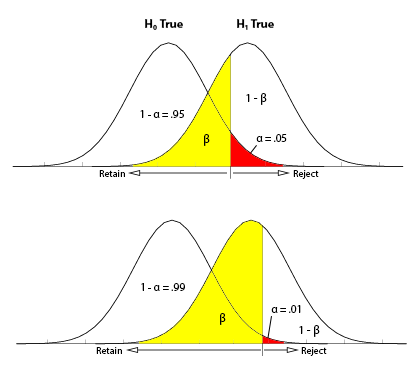
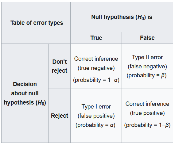
A Type I Error occurs when a researcher rejects a null hypothesis that is actually true; the researcher concludes that a treatment has an effect when it actually doesn’t. This happens when a researcher unknowingly obtains an extreme, non-representative sample. This goes back to alpha level: it’s the probability that the test will lead to a Type I error if the null hypothesis is true.

A Type II Error occurs when a researcher fails to reject the null hypothesis that is really false; this means that the hypothesis test has failed to detect a real treatment effect. This happens when the sample mean is not in the critical region even though the treatment has had an effect on the sample. Usually, this means that the effect of the treatment was small, but it’s still there. The probability of a Type II error is represented by beta

A result is said to be significant or statistically significant if it is very unlikely to occur when the null hypothesis is true. That is, the result is sufficient to reject the null hypothesis. For instance, two means can be significantly different from one another.

Factors that Influence and Assumptions of Hypothesis Testing

Assumptions of Hypothesis Testing:

• Random sampling: it is assumed that the participants used in the study were selected randomly so that we can confidently generalize our findings from the sample to the population.
• Independent observation: two observations are independent if there is no consistent, predictable relationship between the first observation and the second.
  The value of σ is unchanged by the treatment; if the population standard deviation is unknown, we assume that the standard deviation for the unknown population (after treatment) is the same as it was for the population before treatment. There are ways of checking to see if this is true in SPSS or Excel.
• Normal sampling distribution: in order to use the unit normal table to identify the critical region, we need the distribution of sample means to be normal (which means we need the population to be distributed normally and/or each sample size needs to be 30 or greater based on what we know about the central limit theorem).

Factors that influence hypothesis testing:

• The variability of the scores, which is measured by either the standard deviation or the variance. The variability influences the size of the standard error in the denominator of the z-score.
• The number of scores in the sample. This value also influences the size of the standard error in the denominator.

Test statistic: indicates that the sample data are converted into a single, specific statistic that is used to test the hypothesis (in this case, the z-score statistic).

Directional Hypotheses and Tailed Tests

In a directional hypothesis test, also known as a one-tailed test, the statistical hypotheses specify with an increase or decrease in the population mean. That is, they make a statement about the direction of the effect.

The Hypotheses for a Directional Test:

• H0: The test scores are not increased/decreased (the treatment doesn’t work)
• H1: The test scores are increased/decreased (the treatment works as predicted)

Because we’re only worried about scores that are either greater or less than the scores predicted by the null hypothesis, we only worry about what’s going on in one tail meaning that the critical region only exists within one tail. This means that all of the alpha is contained in one tail rather than split up into both (so the whole 5% is located in the tail we care about, rather than 2.5% in each tail). So before, we cared about what’s going on at the 0.025 mark of the unit normal table to look at both tails, but now we care about 0.05 because we’re only looking at one tail.

A one-tailed test allows you to reject the null hypothesis when the difference between the sample and the population is relatively small, as long as that difference is in the direction that you predicted. A two-tailed test, on the other hand, requires a relatively large difference independent of direction. In practice, researchers hypothesize using a one-tailed method but base their findings off of whether the results fall into the critical region of a two-tailed method. For the purposes of this class, make sure to calculate your results using the test that is specified in the problem.

Effect Size

A measure of effect size is intended to provide a measurement of the absolute magnitude of a treatment effect, independent of the size of the sample(s) being used. Usually done with Cohen’s d. If you imagine the two distributions, they’re layered over one another. The more they overlap, the smaller the effect size (the means of the two distributions are close). The more they are spread apart, the greater the effect size (the means of the two distributions are farther apart).

Statistical Power

The power of a statistical test is the probability that the test will correctly reject a false null hypothesis. It’s usually what we’re hoping to get when we run an experiment. It’s displayed in the table posted above. Power and effect size are connected. So, we know that the greater the distance between the means, the greater the effect size. If the two distributions overlapped very little, there would be a greater chance of selecting a sample that leads to rejecting the null hypothesis.

This chapter was originally posted to the Math Support Center blog at the University of Baltimore on June 11, 2019.