7 Comparing Means: Independent Measures One-Way ANOVA

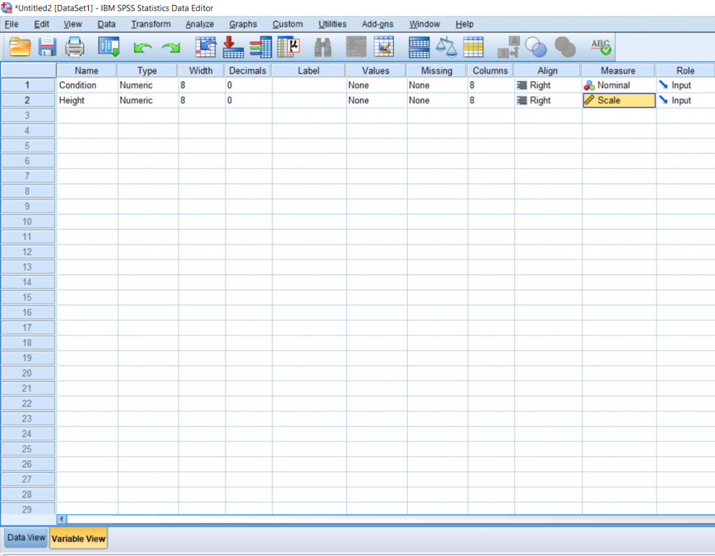
Just like an independent samples t-test, an Independent measures one-way ANOVA uses independent subjects for each level/condition within an independent variable. In this example, we’re growing plants. In Variable View, I’ve made the independent variable Condition (in this case the amount of water I’ll be giving to the plants) and the dependent variable Height.

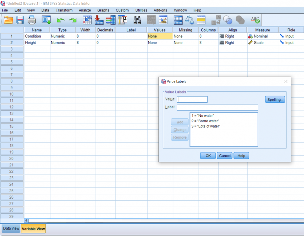
Next, it’s important to label the levels of your independent variable, so I clicked the cell under Values and assigned the numbers 1, 2, and 3 a condition: no water, some water, and a lot of water.

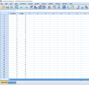
Then, I just put my data in Data View, with the Condition column full of the numbers representing the different conditions and the Height column full of the measured heights of each plant.

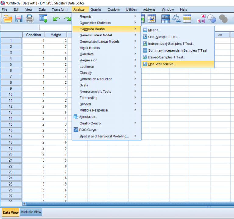
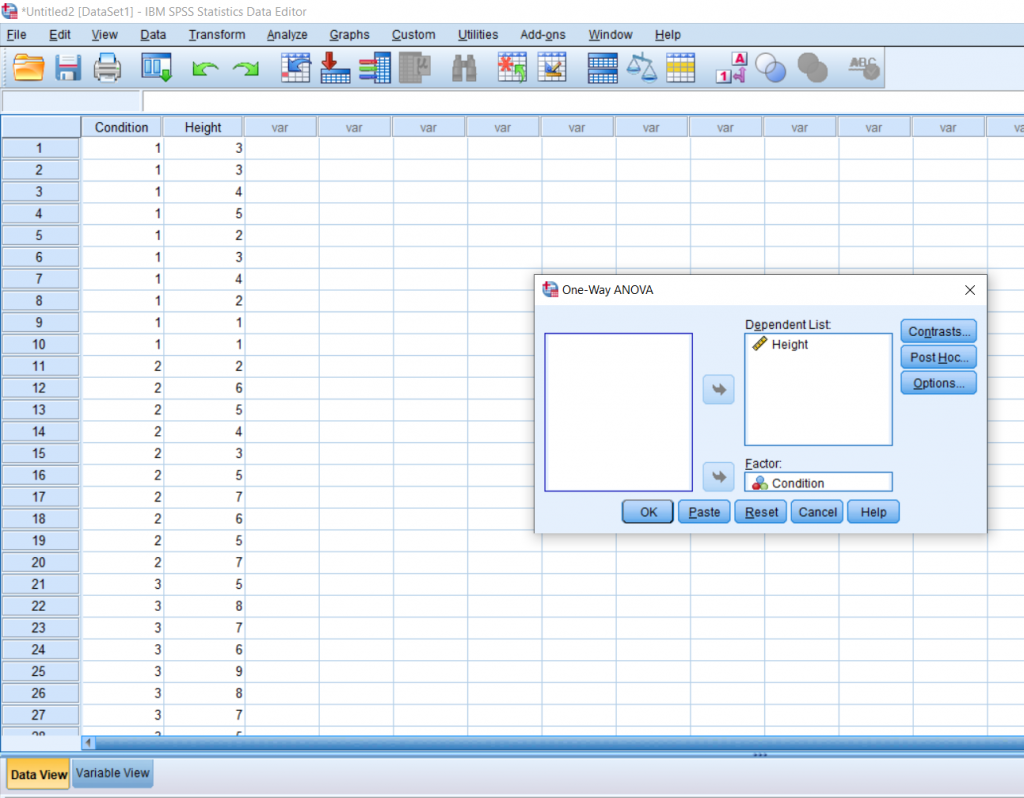
To conduct the test, click Analyze at the top, hover over Compare means, and then click One-Way ANOVA.

You’ll be greeted with a pop-up asking you to arrange the variables you would like to test. The dependent variable goes in the top box and the independent variable goes in the bottom box. Then, click the Post Hoc box.

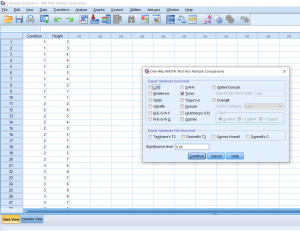
You will be greeted by another pop-up. Here you can click the kind of post hoc test you would like to run. Tukey seems to be pretty popular, so that’s the one I chose. Then, click Continue.

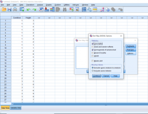
Once back to the main pop-up, then click Options. Here you’ll be able to add in descriptive statistics (like mean, SD, etc.) and a Homogeneity of Variance test, which may be important to report depending on what your professor is asking for. Then, click continue and finally OK.

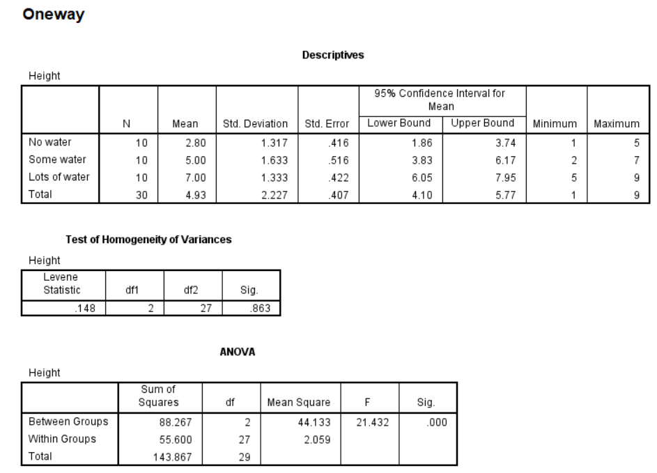
Your output will look something like this. First is always the descriptives. The next box is the results of the test of homogeneity of variances. Remember, this is the one that we don’t want to be significant; we want there to be no difference between the groups. Looking under Sig, we can see that our p-value is greater than 0.05 so we’re in the clear! The third box shows us the result of our analysis overall. Here, our F-value is 21.4 and we have a p-value of less than 0.01, which means that there is definitely a difference somewhere between these three conditions.

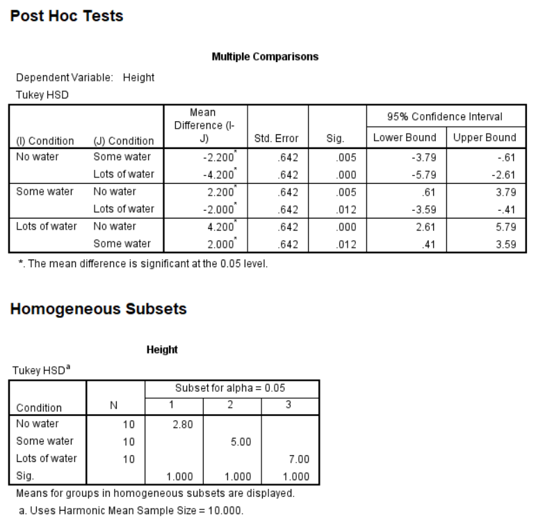
Moving on the Post Hoc, each box compares one group with the other group. So as well can see, no water and some water are significantly different, and no water and lots of water are significantly different (remember that stars indicate significance). We’ve compared conditions 1 and 2 and conditions 1 and 3, but we still need to compare 2 and 3, so we move down to the next box and see that some water and lots of water are also significantly different. Make sure to report all of these differences. To know which groups are significantly less than or greater than others, refer to the descriptive statistics at the top (specifically the means).

This chapter was originally posted to the Math Support Center blog at the University of Baltimore on September 10, 2019.