Spatial Analysis and Mapping with R
6 Spatial Analysis—Part 2
In the previous section we have created maps that show the locations of vaccination sites in rural and urban census tracts.
That required us to:
- filter spatial objects,
- identify and extract spatial feature based on their spatial relation to other spatial features, and
- map (visualize) these features.
In this section we expand our analysis and assess rural communities in a selected county in Maryland and Baltimore City for the potential presence of vaccination deserts. Per our definition, a low-income census tract qualifies as a vaccination desert if 33% of its area is outside a 0.5 mile (urban) or 10 mile (rural) range of the vaccination site (Section 1.1).
Conceptually we need to identify:
- low-income census tracts that are outside of a certain range of a vaccination site, and
- low-income tracts that have less than 33% of their area within the range of a vaccination site.
To identify these tracts, we need to further manipulate spatial objects, including:
- merge spatial features,
- buffer,
- clip, and
- perform simple mathematical operations on spatial features.
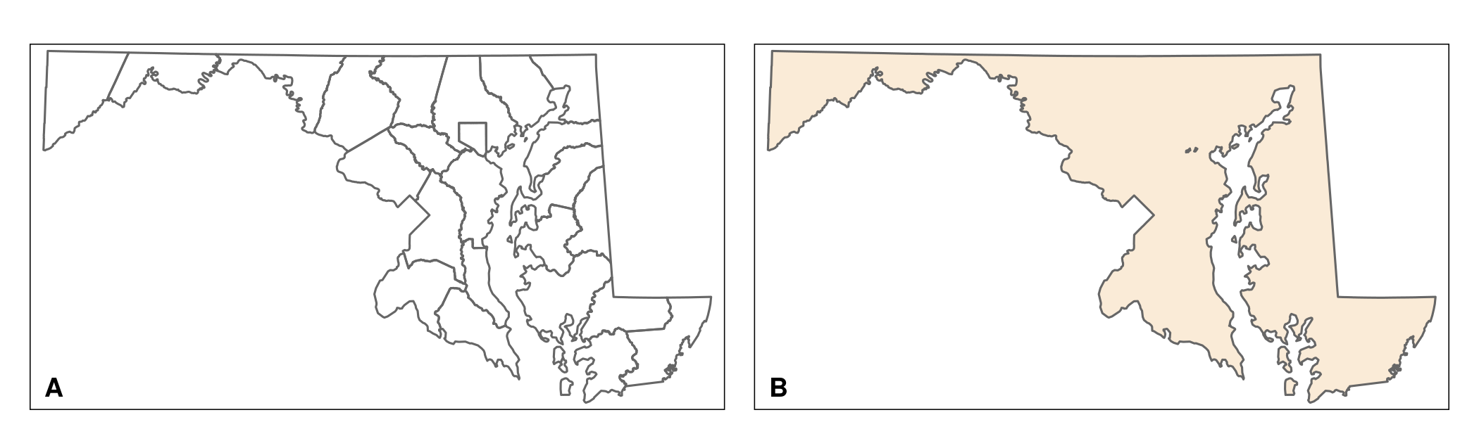
Before we continue, let us create a Maryland state boundary map and a map containing county boundaries. For the latter, read in the shapefile MD_counties_CT.shp. This map contains boundaries of the counties of Maryland. I created the file by extracting all counties from the census tract map (MD_CensusTracts_6487), and unifying the census tracts of each county. The Maryland state boundary map is created by unifying the census tracts of the entire state. The following script produces these maps that should look similar to the maps in Figure 6.1.
MD_counties <- st_read("data/MD_counties_CT.shp")

# draw Map (Fig. 6.1 A)
map_MD_counties <- tm_shape(MD_counties) +
                   tm_borders()
map_MD_counties

# create MD_state (Fig. 6.1 B)
MD_state <- st_union(MD_counties)

# draw Map
map_MD_state <- tm_shape(MD_state) +
                   tm_fill(col = "antiquewhite") +
                   tm_borders()
map_MD_state
6.1 Identification of Possible Rural Vaccination Deserts
To identify areas with limited access to vaccination sites, we first create a 10-mile buffer around all Maryland vaccination sites (listed in VaccineSites_6487) with the function st_buffer(). The CRS of our maps uses meter. Thus, we need to convert miles to meter. One mile is approximately 1.690344 meters. Ten miles are therefore 16,093 meters, which is provided to the dist argument of st_buffer(). We join (unify) overlapping buffers with st_union(), and crop (clip) the ten mile ranges with st_intersection() to the state boundaries of Maryland.
# create a 10 mi buffer
vac_10mi <- st_buffer(VaccineSites_6487, dist = 1.609344*1e04)

# join/unify overlapping buffers
vac_10mi_union <- st_union(vac_10mi)

# clip/crop
vac_10mi_state <- st_intersection(MD_state, vac_10mi_union)
Next we plot Maryland’s vaccination sites with the ten-mile buffer onto the counties “base map” (map_MD_counties). The alpha argument of the tm_fill() function sets a transparency level. One would mean no transparency (100% opacity), and zero 100% transparency (0% opacity). We set it to 65% (alpha = 0.35). The code produces a map similar to Figure 6.2.
# draw map
map_vac_10mi_md <- map_MD_counties +
                   tm_shape(vac_10mi_state) +
                   tm_fill(col = "orange",
                               alpha = 0.35) +
                   tm_borders(col = "red") +
                   map_VaccineSites

map_vac_10mi_md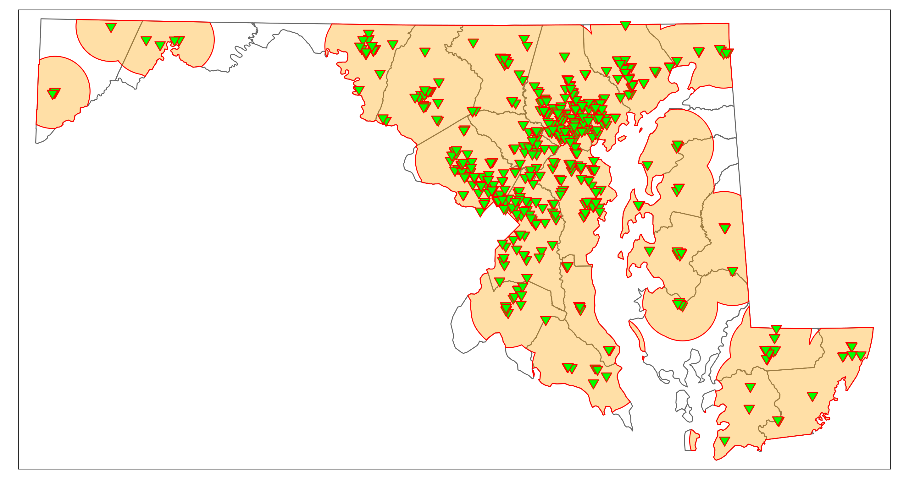
Now we identify low-income rural census tracts. We subset MD_CensusTracts_6487 for Urban == 0 and LowIncomeTracts == 1.
rural_LowIncome <- subset(MD_CensusTracts_6487, Urban == 0 & LowIncomeTracts == 1)

rural_LowIncome
## Simple feature collection with 55 features and 13 fields
## geometry type: MULTIPOLYGON
## dimension: XY
## bbox: xmin: 185230.9 ymin: 27801.06 xmax: 547910.5 ymax: 230941.9
## projected CRS: NAD83(2011) / Maryland
## First 10 features:
## CensusTract GEO_ID STATE COUNTY TRACT NAME LSAD
## 1 24001000100 1400000US24001000100 24 001 000100 1 Tract
## 2 24001000200 1400000US24001000200 24 001 000200 2 Tract
## 3 24001000300 1400000US24001000300 24 001 000300 3 Tract
## 15 24001001502 1400000US24001001502 24 001 001502 15.02 Tract
## 16 24001001503 1400000US24001001503 24 001 001503 15.03 Tract
## 20 24001001900 1400000US24001001900 24 001 001900 19 Tract
## 21 24001002000 1400000US24001002000 24 001 002000 20 Tract
## 23 24001002200 1400000US24001002200 24 001 002200 22 Tract
## 299 24005451900 1400000US24005451900 24 005 451900 4519 Tract
## 353 24009860702 1400000US24009860702 24 009 860702 8607.02 Tract
## CENSUSAREA County Urban POP2010 LowIncomeTracts HUNVFlag
## 1 187.937 Allegany 0 3718 1 0
## 2 48.067 Allegany 0 4564 1 0
## 3 8.656 Allegany 0 2780 1 0
## 15 9.148 Allegany 0 2055 1 0
## 16 11.539 Allegany 0 1968 1 0
## 20 24.855 Allegany 0 2623 1 0
## 21 26.800 Allegany 0 5552 1 1
## 23 23.497 Allegany 0 3874 1 0
## 299 5.187 Baltimore 0 2445 1 0
## 353 9.430 Calvert 0 2974 1 0
## geometry
## 1 MULTIPOLYGON (((277992.7 21...
## 2 MULTIPOLYGON (((252677.1 22...
## 3 MULTIPOLYGON (((252464.7 22...
## 15 MULTIPOLYGON (((243626.5 22...
## 16 MULTIPOLYGON (((241785.2 22...
## 20 MULTIPOLYGON (((234463.9 22...
## 21 MULTIPOLYGON (((241888.4 21...
## 23 MULTIPOLYGON (((231767.6 19...
## 299 MULTIPOLYGON (((456497.8 17...
## 353 MULTIPOLYGON (((434677 1017...There are 55 census tracts that qualify. The code below plots these tracts onto the map (Figure 6.3).
map_Rural_LowIncome_md <- map_MD_counties +
                          tm_shape(rural_LowIncome) +
                          tm_fill(col = "red",
                                  alpha = 0.75) +
                          tm_shape(vac_10mi_state) +
                          tm_fill(col = "orange",
                                  alpha = 0.5) +
                          tm_borders(col = "blue") +
                          map_VaccineSites

map_Rural_LowIncome_md
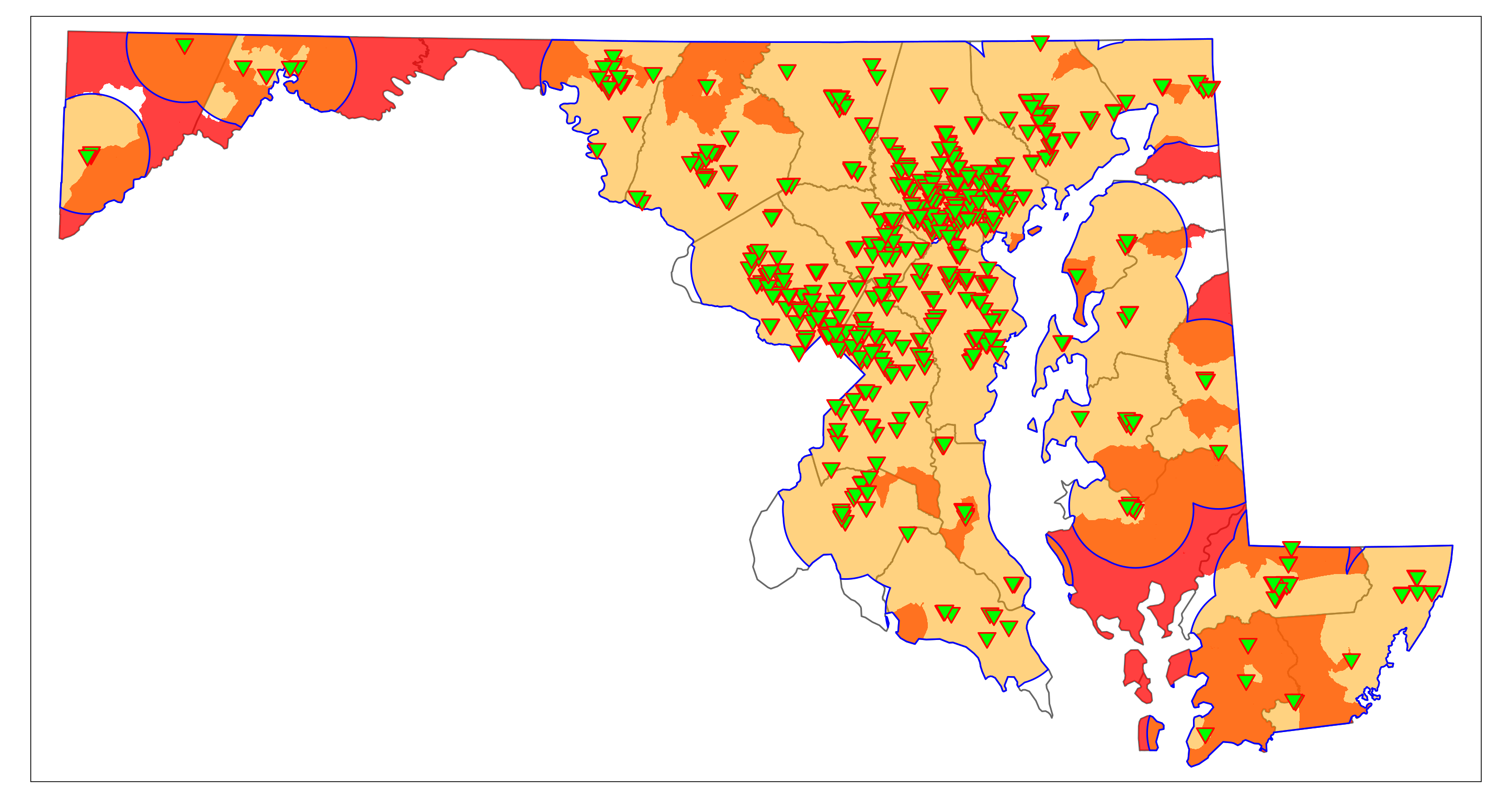
We can narrow down the rural regions that may contain vaccination deserts by identifying rural low-income areas that are outside the 10-mile range of a vaccination site. The function st_difference() clips features that do not intersect with other features or are within other features. (Note that the code may produce a warning that can be ignored). The resulting plot should be similar to Figure 6.4. It shows rural areas (not census tracts) that would have limited access to vaccination sites in “hot pink.” They are mainly located on the Eastern Shore (parts of Dorchester, Queen Anne’s, and Kent County) and in Western Maryland (parts of Washington, Allegany, and Garrett County).
rural_vac_desert <- st_difference(rural_LowIncome, vac_10mi_state)

map_Rural_vac_desert <- map_MD_counties +
                        tm_shape(rural_vac_desert) +
                        tm_fill(col = "hotpink",
                                alpha = 0.75) +
                        tm_shape(vac_10mi_state) +
                        tm_fill(col = "orange",
                                alpha = 0.5) +
                        tm_borders(col = "blue") +
                        map_VaccineSites
map_Rural_vac_desert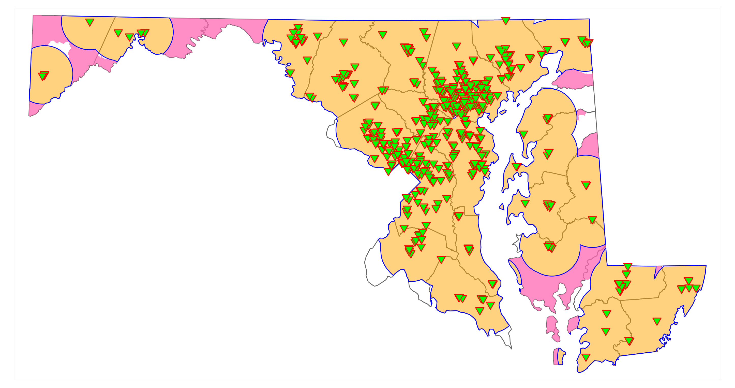
6.2 Possible Vaccination Deserts in Garrett County
The analysis above suggests that Garrett County in Western Maryland may have rural vaccination deserts, which warrants further analysis. Before we continue, we create a basemap for Garrett County that allows us to map possible vaccination deserts in Garrett County. The code below extracts Garrett County from MD_CensusTracts_6487 using the County variable. It unifies the census tracts and plots a map. The plot should look similar to Figure 6.5 A.
Garrett_CensusTracts <- subset(MD_CensusTracts_6487, County == "Garrett")
Garrett_CensusTracts

Garrett_County <- st_union(Garrett_CensusTracts)

map_Garrett <- tm_shape(Garrett_County) +
               tm_fill(col = "antiquewhite") +
               tm_borders(col = "black")
map_Garrett
Next, we extract and map rural low-income tracts, that are highlighted in red. For reference, all census tracts are outlined (Figure 6.5 B).
Garrett_RuralLowIncome <- subset(Garrett_CensusTracts, Urban == 0 & LowIncomeTracts == 1)
Garrett_RuralLowIncome

map_Garrett_RuralLowIncome <- map_Garrett +
                              tm_shape(Garrett_CensusTracts) +
                              tm_borders(col = "black") +
                              tm_shape(Garrett_RuralLowIncome) +
                              tm_fill(col = "orange") +
                              tm_borders(col = "black")
map_Garrett_RuralLowIncome
Five of the seven census tracts in Garrett County qualify as rural low-income tracts. Next, we identify vaccination sites located in Garrett County. To identify areas with limited access to these sites we create again a 10-mile buffer around the Garrett County vaccination sites, join overlapping buffers, and clip the 10-mile buffers to the boundaries of Garrett County. For reference we label the tracts with their names (listed in the variable NAME) (Figure 6.5 C).
# Identify vaccination sites
vac_Garrett <- st_intersection(VaccineSites_6487, Garrett_County)

# Create a 10 mile buffer around vaccination sites
vac_Garrett_10mi <- st_buffer(vac_Garrett, dist = 1.690344*1e04)

# unify
vac_Garrett_10mi <- st_union(vac_Garrett_10mi)

# Clip to Garrett County Boundaries
vac_Garrett_10mi_clipped <- st_intersection(Garrett_County, vac_Garrett_10mi)

# map
# Garrett County Vaccine Sites
map_vac_Garrett <- tm_shape(vac_Garrett) +
                   tm_symbols(shape = 25,
                              size = 0.75,
                              col = "green",
                              border.col = "red")

map_Garrett_RuralLowIncome_10mi <- map_Garrett_RuralLowIncome +
                                   tm_shape(vac_Garrett_10mi_clipped) +
                                   tm_fill(col = "purple",
                                           alpha = 0.5) +
                                   map_vac_Garrett
map_Garrett_RuralLowIncome_10mi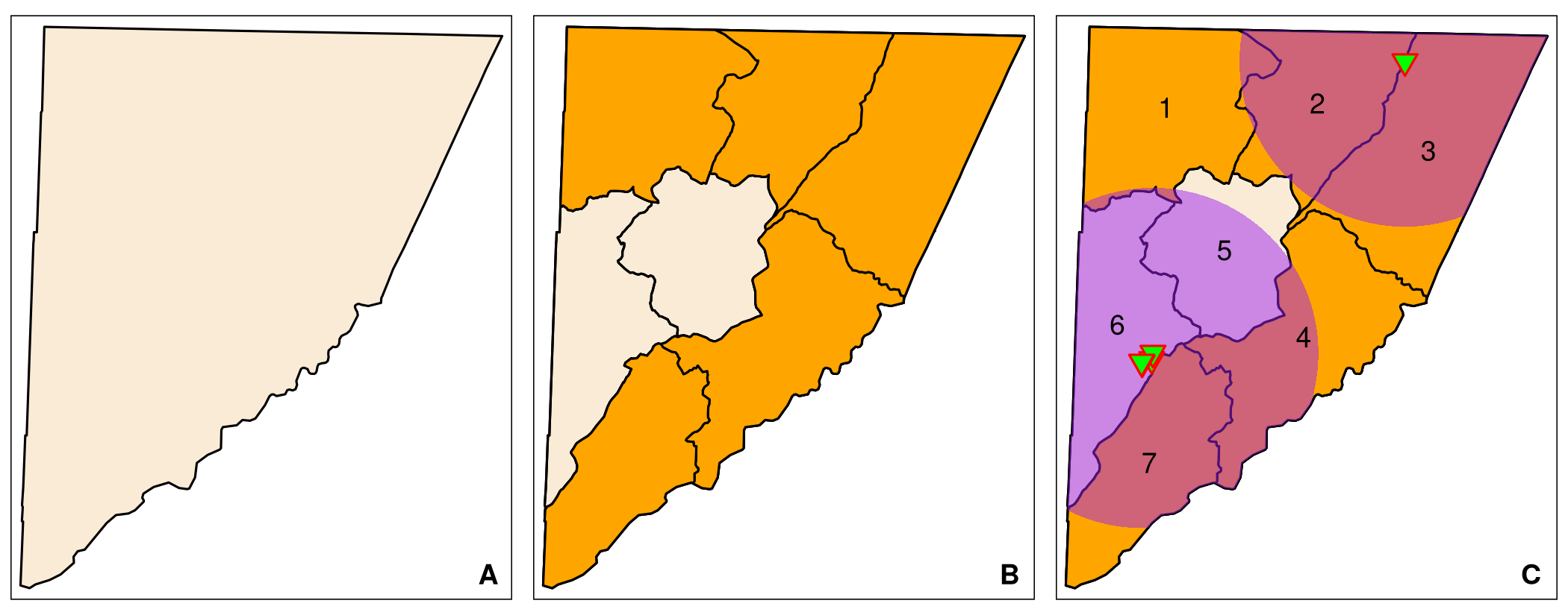
Garrett County has five rural low-income tracts: tracts 1–4, and tract 7. Tracts 2–4 and 7 have large areas that are within the range of a vaccination site. Tract 1 has only two small sections that are within the range (Figure 6.5 C).
As discussed in Section 1.1, a low-income census tract should have at least 33% of its area outside of the range of a vaccination site to be flagged as a possible vaccination desert. Remember however that this definition has its limitations. It suggests that residential housing is evenly distributed throughout the census tract. This is likely not true for many rural areas.
Regardless, let’s determine the relative sizes of the low-income census tracts sections that are outside of the range of a vaccination site. To do so, we first identify the sections that are within the range of a vaccination site, and determine their sizes. We use st_intersection() to extract the portions of the census tracts that is within the range of a vaccination site. Note that the low-income census tracts are listed first, followed by the 10-mile vaccination site buffer. Also, st_intersection() will issue a warning that can be ignored. The resulting spatial object is assigned to vac_assess. Next, we calculate the area of the spatial features with st_area() (and assign the outcome to vac_access_area). Then we calculate the total area of the low-income census tracts (st_area(Garrett_RuralIncome)) and assign the output to the object Garrett_RuralLowIncome_area.
Since all five low-income tracts of Garrett County overlap with the 10-mile range of a vaccination site, we can calculate the relative area of a low-income tract that is outside the reach of a vaccination site by dividing vac_access_area by Garrett_RuralLowIncome_area. The quotient (result of the division) is converted into a vector (function as.vector()) and subtracted from one. The final ratio is assigned to a new variable (outside_range_ratio) to the Garrett_RuralLowIncome_vac_area created beforehand.
# determine region within range
vac_access <- st_intersection(Garrett_RuralLowIncome, vac_Garrett_10mi)
## Warning: attribute variables are assumed to be spatially constant throughout all
## geometriesvac_access_area <- st_area(vac_access)
vac_access_area ## Units: [m^2]
## [1] 21235139 190265302 267057684 137166602 177668272# calcualting total area of each census tract (low income)
Garrett_RuralLowIncome_area <- st_area(Garrett_RuralLowIncome)
Garrett_RuralLowIncome_area## Units: [m^2]
## [1] 275216882 208291591 323333623 268461042 214505992# copy Garrett_RuralLowIncome
Garrett_RuralLowIncome_vac_area <- Garrett_RuralLowIncome
# Calculate area outside of the range
Garrett_RuralLowIncome_vac_area$outside_range_ratio <- 1 - as.vector(vac_access_area/Garrett_RuralLowIncome_area)
Garrett_RuralLowIncome_vac_area## Simple feature collection with 5 features and 14 fields
## geometry type: MULTIPOLYGON
## dimension: XY
## bbox: xmin: 185230.9 ymin: 173522.8 xmax: 234427.1 ymax: 230941.9
## projected CRS: NAD83(2011) / Maryland
## CensusTract GEO_ID STATE COUNTY TRACT NAME LSAD CENSUSAREA
## 530 24023000100 1400000US24023000100 24 023 000100 1 Tract 105.372
## 531 24023000200 1400000US24023000200 24 023 000200 2 Tract 80.293
## 532 24023000300 1400000US24023000300 24 023 000300 3 Tract 124.156
## 533 24023000400 1400000US24023000400 24 023 000400 4 Tract 102.178
## 536 24023000700 1400000US24023000700 24 023 000700 7 Tract 82.476
## County Urban POP2010 LowIncomeTracts HUNVFlag
## 530 Garrett 0 4003 1 1
## 531 Garrett 0 3937 1 1
## 532 Garrett 0 2857 1 0
## 533 Garrett 0 3337 1 0
## 536 Garrett 0 5726 1 1
## geometry outside_range_ratio
## 530 MULTIPOLYGON (((187332 2221... 0.92284216
## 531 MULTIPOLYGON (((202819.1 23... 0.08654353
## 532 MULTIPOLYGON (((222190.9 20... 0.17404914
## 533 MULTIPOLYGON (((205719.8 18... 0.48906329
## 536 MULTIPOLYGON (((197757.6 18... 0.17173283We then extract low-income tracts with an outside_range_ratio larger than 33% (0.33), which represent possible vaccination deserts.
# subset for vaccination deserts
Garrett_RuralVacDeserts <- subset(Garrett_RuralLowIncome_vac_area, outside_range_ratio > 0.33)
Garrett_RuralVacDeserts
## Simple feature collection with 2 features and 14 fields
## geometry type: MULTIPOLYGON
## dimension: XY
## bbox: xmin: 186998.7 ymin: 183652.7 xmax: 222098.7 ymax: 230941.9
## projected CRS: NAD83(2011) / Maryland
## CensusTract GEO_ID STATE COUNTY TRACT NAME LSAD CENSUSAREA
## 530 24023000100 1400000US24023000100 24 023 000100 1 Tract 105.372
## 533 24023000400 1400000US24023000400 24 023 000400 4 Tract 102.178
## County Urban POP2010 LowIncomeTracts HUNVFlag
## 530 Garrett 0 4003 1 1
## 533 Garrett 0 3337 1 0
## geometry outside_range_ratio
## 530 MULTIPOLYGON (((187332 2221... 0.9228422
## 533 MULTIPOLYGON (((205719.8 18... 0.4890633The results suggest that there are two rural low-income census tracts in Garrett County that have limited access to vaccination sites (more than 33% of their area is outside the range of a vaccination site): tract 1 and tract 4. These potential vaccination deserts are mapped with the code below, which produces plot a similar to Figure 6.6.
# map
map_Garrett_RuralVacDeserts <- map_Garrett +
                               tm_shape(Garrett_CensusTracts) +
                               tm_borders(col = "black") +
                               tm_shape(Garrett_RuralLowIncome) +
                               tm_polygons(col = "orange") +
                               tm_shape(Garrett_RuralVacDeserts) +
                               tm_polygons(col = "red") +
                               map_vac_Garrett +
                               tm_add_legend(type = "symbol",
                                             shape = c(22, 22, 25),
                                             size = c(0.9, 0.9, 0.65),
                                             col = c("orange", "red", "green"),
                                             border.col = c("black", "black", "red"),
                                             label = c("Rural Low-income Tract",
                                                       "Potential Vaccination Desert",
                                                       "COVID-19 Vaccination Site")) +
                             tm_legend(position = c(0.475, 0.02),
                                       width = 0.6) +
                             tm_layout(legend.text.size = 0.85)

map_Garrett_RuralVacDeserts

#save map
tmap_save(map_Garrett_RuralVacDeserts, filename = "figures/map_Garrett_RuralVacDeserts.png")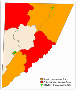
Note that you may need to adjust the position of the legend manually for the saved file. I adjusted the legend position as follows to save the map to my liking (just replace the lines containing the tm_legend(position …)).
tm_legend(position = c(0.65, 0.02),
                       width = 0.6) +
6.3 Possible Vaccination Deserts in Baltimore City
We can use a similar approach to assess whether Baltimore City has “COVID-19 Vaccination Deserts.” Of course, there are some modifications necessary.
- Remember, in an urban setting, we defined a limited-access census tract as a census tract where more than 33% of the area is outside of a 0.5 mile range to a vaccination site (0.5 mile is roughly 800 m). Thus, instead of creating a 10-mile buffer around vaccination sites, we create a 0.5 mile (800 m) buffer.
- Baltimore City is surrounded by other (Maryland) counties, in which Baltimore City residents can get vaccinated. Therefore, vaccination sites will be clipped to Baltimore City limits that are “expanded” by 800 m.
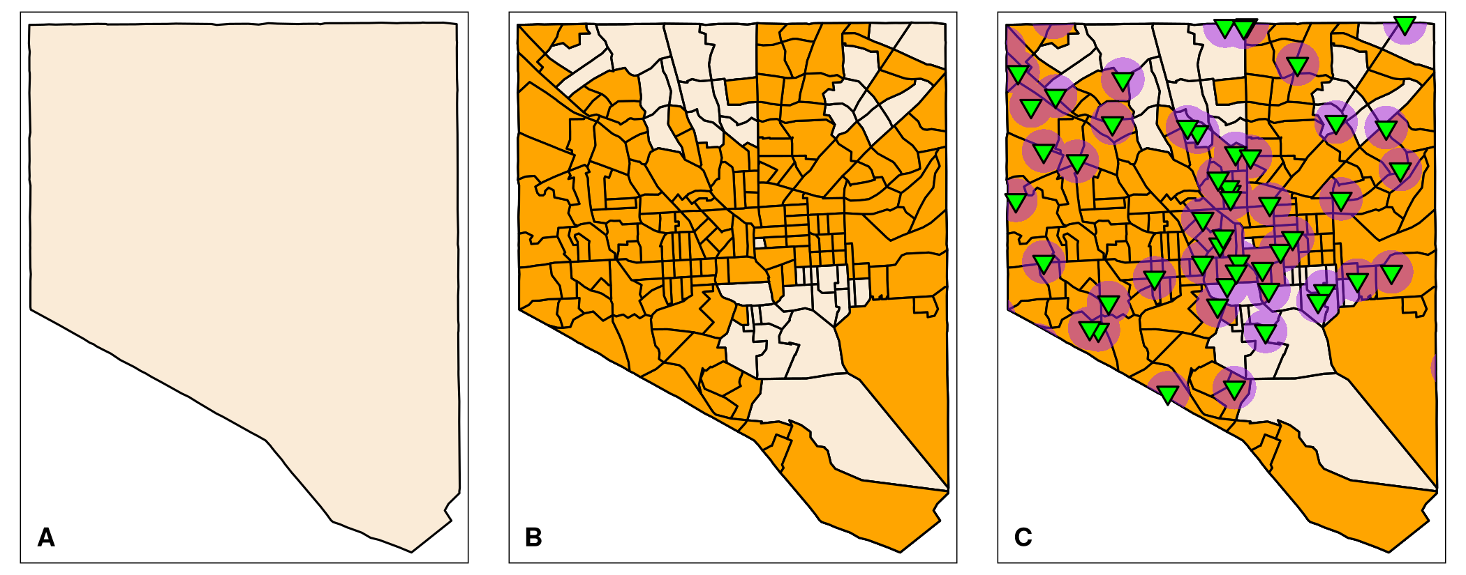
- As you will see, in contrast to Garrett County, Baltimore City has low-income tracts that are outside of the 0.5 miles range of vaccination sites (Figure 6.7 C), which we have to account for.
The first steps (up to mapping low-income tracts and buffered vaccination sites) in general follow the example we used for Garrett County:
- We create a base map for Baltimore City and a map showing census tracts.
- We extract low-income tracts and double check that we only have urban tracts.
- We create a 800 m buffer around Baltimore City limits and identify vaccination sites that are within the extended Baltimore City limits.
- We create a 800 m buffer around the vaccination sites and clip the buffered sites to the city limits (for aesthetics).
- We plot Baltimore City’s census tracts, low-income census tracts, and buffered vaccination sites.
# Create Baltimore City map
# From Census Tract Map
BC_CensusTracts <- subset(MD_CensusTracts_6487, County == "Baltimore City")

# Baltimore City outline
BC <- st_union(BC_CensusTracts)

# Map BC (Figure 6.7 A)

map_BC <- tm_shape(BC) +
          tm_fill(col = "antiquewhite") +
          tm_borders(col = "black")
map_BC
# Extract low income census tracts.
# check if non urban tracts are present.
subset(BC_CensusTracts, Urban == 0)  # just to be sure
## Simple feature collection with 0 features and 13 fields
## bbox:           xmin: NA ymin: NA xmax: NA ymax: NA
## projected CRS:  NAD83(2011) / Maryland
##  [1] CensusTract     GEO_ID          STATE           COUNTY
##  [5] TRACT           NAME            LSAD            CENSUSAREA
##  [9] County          Urban           POP2010         LowIncomeTracts
## [13] HUNVFlag        geometry
##  (or 0-length row.names)
# <0 rows>, we are good to go
# Extract LowIncomeTracts
BC_LowIncome <- subset(BC_CensusTracts, LowIncomeTracts == "1")

# Map census tracts, highlight low-income census tracts orange (Fig. 6.7 B)

map_BC_LowIncome <- map_BC +
                    tm_shape(BC_CensusTracts) +
                    tm_borders(col = "black") +
                    tm_shape(BC_LowIncome) +
                    tm_fill(col = "orange") +
                    tm_borders(col = "black")
map_BC_LowIncome
# Create 800 m buffer for Baltimore City
BC_800m <- st_buffer(BC, dist = 800)

# Identify Vaccination Sites in BC (for mapping sites); ignore warning
vac_BC <- st_intersection(VaccineSites_6487, BC)

# Identify Vaccination Sites within "expanded" City; ignore warning
vac_BC_ext <- st_intersection(VaccineSites_6487, BC_800m)

# Create 0.5 mi (800m) buffer
vac_BC_800m <- st_buffer(vac_BC_ext, dist = 800)

# Unify
vac_BC_800m <- st_union(vac_BC_800m)

# Clip to BC boundaries (NOT BC_800m)
vac_BC_800m_clipped <- st_intersection(BC, vac_BC_800m)

# Map Vaccination Sites and buffer, only map sites in the city (Figure 6.7 C)
map_vac_BC <- tm_shape(vac_BC) +
              tm_symbols(shape = 25,
                         size = 0.5,
                         col = "green",
                         border.col = "black")
# map (figure 6.7 C)
map_BC_LowIncome_800m <- map_BC_LowIncome +
                         tm_shape(vac_BC_800m_clipped) +
                         tm_fill(col = "purple",
                                 alpha = 0.5) +
                         map_vac_BC
map_BC_LowIncome_800m
The R script produces maps similar to the plots in Figure 6.7 A–C. Indeed, Baltimore City has quite a few low-income tracts that are outside the 0.5 mile range of vaccination sites. These by definition are possible vaccination deserts. We need to separate them from the low-income tracts that are within the range of vaccination sites. Otherwise, we cannot calculate the area that overlap. The package dplyr has the function anti_join() that removes rows of a data frame if the rows are present in another data frame. However, the function does not work with 2 sf objects. The 2nd object needs to be a non spatial data frame.
To separate the low-income tracts that share some area with the buffered vaccination sites, we use the following approach.
- We identify the area of the census tracts that overlap with the buffered vaccination site and name these
BC_vac_access. We are using the functionst_intersection(). As the function name implies, a spatial data frame is returned that only contains the intersection of both the census tracts and the buffered vaccination sites (Figure 6.8 A). - We obtain the tracts that do not overlap (the “no-access” tracts) by removing the tracts with access from the overall low-income tracts with the function
dplyr::anti_join(). This possible because insfobjects the functionst_intersection()does not alter non spatial information. - We obtain the entire census tracts that overlap with the buffered vaccination sites. We assign these tracts to the object
BC_withvac_access.
The following R scripts produces a few plots that visualize the above process. The plots are shown in Figure 6.8 A–C. st_intersection() will again give warnings that can be ignored.
#====================================================
# Step 1: identify the area that overlaps
#====================================================

BC_vac_access <- st_intersection(BC_LowIncome, vac_BC_800m_clipped)

# Map BC_vac_access (Fig. 6.8 A)
# create an outline of Low Access census tracts
BC_LowIncome_outline <- st_union(BC_LowIncome)

# base map
BC_LI <- tm_shape(BC_LowIncome_outline) +
      tm_borders(col = "darkorange3",
                 lwd = 1.5) +
      tm_shape(BC_LowIncome_outline) +
      tm_fill(col = "antiquewhite") +
      tm_borders(col = "darkorange3",
               lwd = 1.5)

map_BC_vac_access <- BC_LI +
    tm_shape(BC_vac_access) +  # area of overlap
    tm_fill(col = "purple",
            alpha = 0.25) +
    tm_borders(col = "darkblue")
map_BC_vac_access

#====================================================
# Step 2: identify census tracts that do not overlap
#====================================================

# Remove geometries from BC_vac_access
# drop spatial information from overlap (BC_vac_access
BC_vac_access_nsp <- st_drop_geometry(BC_vac_access)

BC_novac_access <- dplyr::anti_join(BC_LowIncome, BC_vac_access_nsp, by = "NAME")

# Map BC_novac_access (Fig. 6.8 B)
map_BC_novac_access <- BC_LI +
    tm_shape(BC_novac_access) + # tracts w/ no access
    tm_polygons(col = "red")

map_BC_novac_access

#===============================================
# Step 3 get census tracts with access (overlap)
#===============================================

# Remove geometries from BC_novac_access
BC_novac_access_nsp <- st_drop_geometry(BC_novac_access)

# Remove no-access from low-income tract
BC_withvac_access <- dplyr::anti_join(BC_LowIncome, BC_novac_access_nsp, by = "NAME")

# Map BC_withvac_access (Fig. 6.8 C)
map_BC_withvac_access <- BC_LI +
            tm_shape(BC_withvac_access) +
            tm_fill(col = "orange",
                    alpha = 0.5) +
            tm_borders(col = "darkorange3")

map_BC_withvac_access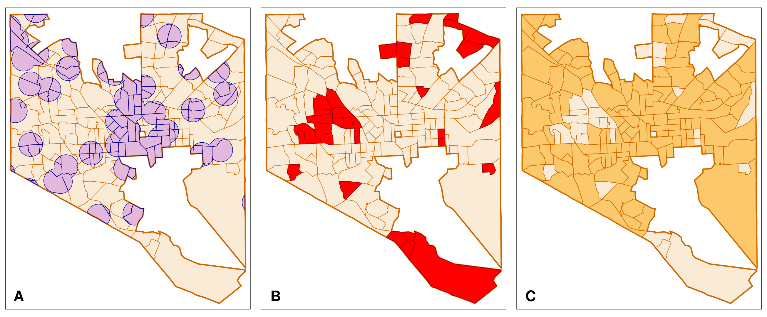
We have two sets of complete low-income census tracts: (1) census tracts that do not overlap (“no-access” low-income tracts; Figure 6.8 B), and (2) those that have areas within the 0.5 mile range to vaccination sites (“with-access” low-income tracts; Figure 6.8 C). These data sets allow us to calculate the portion of the area of a low-income tract that overlaps with the 0.5 mile buffer around vaccination sites. For these calculations it is important that the census tracts in both data frames (BC_vac_access and BC_withvac_access) are in the same order. To verify, we use the function identical(). It tests if two objects are exactly the same. We cannot compare the entire data frames since the geometry columns of the data frames differ. Furthermore, anti_join() from the dplyr package unfortunately does not preserve the row numbers. Instead we compare the entries in the variable GEO_ID as it is unique to each tract.
# check if NAME viable is the same in both data frames
identical(BC_vac_access$GEO_ID, BC_withvac_access$GEO_ID)
## [1] TRUETRUE is returned, confirming that in both data sets the order of the census tracts is identical. We now identify possible low-income tracts with limited-access to vaccination sites following the example of Garrett County. We first divide the area of the intersection (BC_vac_access) by the total area of the tract (BC_withvac_access), then subtract the quotient from 1, and lastly extract tracts that share no more than 33% with the buffer around vaccination sites.
# calculate area of the portions that are within the 0.5 mile range
BC_vac_access_area <- st_area(BC_vac_access)

BC_vac_access_area
## Units: [m^2]
## [1] 426051.567 595722.353 1204742.968 437131.380 1595.308 68083.216
## [7] 420835.141 133338.221 225786.014 326691.483 15006.228 281497.037
## [13] 247188.754 74697.281 38425.821 202105.805 291927.929 251092.218
## [19] 282982.776 327353.482 53235.925 128529.689 534636.724 291398.885
## [25] 354049.787 87394.618 787116.713 544379.226 91860.517 204809.073
## [31] 308259.900 706061.179 356875.579 934568.962 408658.063 270852.756
## [37] 382688.840 503295.282 1020097.808 24903.375 318708.773 26947.737
## [43] 8289.565 507238.123 293322.753 314815.420 593204.994 316978.938
## [49] 259617.680 438479.266 298329.823 783814.209 681257.558 97632.114
## [55] 875160.584 143299.770 12652.807 70685.473 46630.607 276051.933
## [61] 484918.575 283264.985 340923.971 177094.232 160975.836 248396.176
## [67] 92184.117 271324.877 265150.352 386301.387 207259.904 240586.509
## [73] 180069.772 1248149.304 92392.360 130851.261 481958.333 989663.497
## [79] 3416.019 292827.299 74827.221 1723568.441 1051350.778 29350.392
## [85] 1186969.701 541803.150 407432.500 90406.402 44231.254 662949.100
## [91] 1248459.714 173237.048 671154.321 130106.429 606352.391 536479.279
## [97] 10152.565 423422.520 648875.862 1576870.203 171886.689 730677.745
## [103] 311145.862 84521.796 481436.695 801923.164 783199.034 575371.412
## [109] 62320.814 94295.486 305834.031 42781.522 753480.037 940759.662
## [115] 401882.661 46069.995 418841.769 294534.122 426904.915 758439.728
## [121] 1306801.799 2602953.864 1175111.918 1363236.743 113529.070 854045.245
## [127] 228777.089 408589.497 480149.958 924871.056# Calculate total area of each low-income census tracts that intersect with a buffer
BC_withvac_access_area <- st_area(BC_withvac_access)
BC_withvac_access_area## Units: [m^2]
## [1] 427345.4 595722.4 1204743.0 437131.4 257719.1 186938.5
## [7] 429559.1 314502.5 225786.0 326691.5 2299202.9 364736.1
## [13] 863578.2 268338.1 440547.7 251437.0 350511.1 336465.9
## [19] 298794.8 327485.2 659655.6 2031460.0 795632.8 350196.9
## [25] 744957.2 446013.3 844748.8 685535.9 453673.4 304861.7
## [31] 308259.9 706061.2 356875.6 991486.1 408658.1 270852.8
## [37] 532064.0 503295.3 1040072.6 298538.9 362711.1 357715.6
## [43] 2825307.7 904919.4 679703.3 718015.6 593205.0 395240.6
## [49] 391087.0 1090207.3 1455134.1 1489384.5 1691295.7 775813.7
## [55] 938545.1 382271.0 255419.0 398742.1 1050387.4 276051.9
## [61] 487427.0 310599.0 340924.0 234698.9 290125.6 382635.7
## [67] 277363.1 380917.3 265150.4 931568.8 238474.1 398644.6
## [73] 683109.9 1809786.4 1199178.7 288614.6 1082656.5 1477763.3
## [79] 2358753.8 330709.1 975141.6 2585246.1 1283257.1 816551.0
## [85] 2325837.4 2578126.4 1306904.1 2240766.9 1637342.2 1457068.4
## [91] 1632642.9 1025175.6 885456.9 612403.1 885014.5 1236183.8
## [97] 1334571.4 1365204.3 4464233.6 3218863.2 17165266.5 762390.6
## [103] 311481.4 310251.5 972807.3 1097472.2 2177944.3 696604.8
## [109] 1269181.3 681341.4 1132474.6 1085186.7 845572.7 1735994.4
## [115] 566402.8 516018.6 729234.7 924512.3 739565.7 804749.8
## [121] 1418617.5 3493791.3 2414014.1 3224540.7 979278.6 1645592.4
## [127] 553237.0 1819413.2 870269.1 924956.5# copy BC_withvac_access
BC_withvac_access_vac_area <- BC_withvac_access
# calcuate area outside of the range
BC_withvac_access_vac_area$outside_range_ratio <-
1 - as.vector(BC_vac_access_area/BC_withvac_access_area)
BC_withvac_access_vac_area## Simple feature collection with 130 features and 14 fields
## geometry type: MULTIPOLYGON
## dimension: XY
## bbox: xmin: 424860.5 ymin: 172357 xmax: 440631.8 ymax: 189404.6
## projected CRS: NAD83(2011) / Maryland
## First 10 features:
## CensusTract GEO_ID STATE COUNTY TRACT NAME LSAD CENSUSAREA
## 1 24510030100 1400000US24510030100 24 510 030100 301 Tract 0.165
## 2 24510030200 1400000US24510030200 24 510 030200 302 Tract 0.195
## 3 24510040100 1400000US24510040100 24 510 040100 401 Tract 0.463
## 4 24510040200 1400000US24510040200 24 510 040200 402 Tract 0.169
## 5 24510060200 1400000US24510060200 24 510 060200 602 Tract 0.100
## 6 24510060300 1400000US24510060300 24 510 060300 603 Tract 0.072
## 7 24510060400 1400000US24510060400 24 510 060400 604 Tract 0.166
## 8 24510070200 1400000US24510070200 24 510 070200 702 Tract 0.120
## 9 24510070300 1400000US24510070300 24 510 070300 703 Tract 0.088
## 10 24510070400 1400000US24510070400 24 510 070400 704 Tract 0.126
## County Urban POP2010 LowIncomeTracts HUNVFlag
## 1 Baltimore City 1 3065 1 1
## 2 Baltimore City 1 2342 1 0
## 3 Baltimore City 1 4006 1 0
## 4 Baltimore City 1 838 1 0
## 5 Baltimore City 1 3265 1 0
## 6 Baltimore City 1 1800 1 0
## 7 Baltimore City 1 1183 1 1
## 8 Baltimore City 1 3782 1 0
## 9 Baltimore City 1 1042 1 0
## 10 Baltimore City 1 1241 1 0
## geometry outside_range_ratio
## 1 MULTIPOLYGON (((434910.7 17... 0.003027589
## 2 MULTIPOLYGON (((433985.8 18... 0.000000000
## 3 MULTIPOLYGON (((433926.2 18... 0.000000000
## 4 MULTIPOLYGON (((432439.3 18... 0.000000000
## 5 MULTIPOLYGON (((436345.8 18... 0.993809897
## 6 MULTIPOLYGON (((435592.6 18... 0.635798801
## 7 MULTIPOLYGON (((435161.1 18... 0.020309062
## 8 MULTIPOLYGON (((436406 1810... 0.576034505
## 9 MULTIPOLYGON (((435524.7 18... 0.000000000
## 10 MULTIPOLYGON (((435290.8 18... 0.000000000# subset for limited access
BC_limvac_access <- subset(BC_withvac_access_vac_area, outside_range_ratio > 0.33)
BC_limvac_access## Simple feature collection with 75 features and 14 fields
## geometry type: MULTIPOLYGON
## dimension: XY
## bbox: xmin: 424876.1 ymin: 172357 xmax: 440631.8 ymax: 189404.6
## projected CRS: NAD83(2011) / Maryland
## First 10 features:
## CensusTract GEO_ID STATE COUNTY TRACT NAME LSAD CENSUSAREA
## 5 24510060200 1400000US24510060200 24 510 060200 602 Tract 0.100
## 6 24510060300 1400000US24510060300 24 510 060300 603 Tract 0.072
## 8 24510070200 1400000US24510070200 24 510 070200 702 Tract 0.120
## 11 24510080101 1400000US24510080101 24 510 080101 801.01 Tract 0.894
## 13 24510080200 1400000US24510080200 24 510 080200 802 Tract 0.332
## 14 24510080301 1400000US24510080301 24 510 080301 803.01 Tract 0.104
## 15 24510080302 1400000US24510080302 24 510 080302 803.02 Tract 0.170
## 21 24510090100 1400000US24510090100 24 510 090100 901 Tract 0.254
## 22 24510090200 1400000US24510090200 24 510 090200 902 Tract 0.671
## 25 24510090500 1400000US24510090500 24 510 090500 905 Tract 0.286
## County Urban POP2010 LowIncomeTracts HUNVFlag
## 5 Baltimore City 1 3265 1 0
## 6 Baltimore City 1 1800 1 0
## 8 Baltimore City 1 3782 1 0
## 11 Baltimore City 1 3881 1 1
## 13 Baltimore City 1 1585 1 0
## 14 Baltimore City 1 2084 1 0
## 15 Baltimore City 1 2937 1 1
## 21 Baltimore City 1 4251 1 1
## 22 Baltimore City 1 3243 1 0
## 25 Baltimore City 1 1964 1 1
## geometry outside_range_ratio
## 5 MULTIPOLYGON (((436345.8 18... 0.9938099
## 6 MULTIPOLYGON (((435592.6 18... 0.6357988
## 8 MULTIPOLYGON (((436406 1810... 0.5760345
## 11 MULTIPOLYGON (((435823.6 18... 0.9934733
## 13 MULTIPOLYGON (((435460.7 18... 0.7137622
## 14 MULTIPOLYGON (((436130 1816... 0.7216300
## 15 MULTIPOLYGON (((436252.3 18... 0.9127772
## 21 MULTIPOLYGON (((433659.8 18... 0.9192974
## 22 MULTIPOLYGON (((435030.3 18... 0.9367304
## 25 MULTIPOLYGON (((434050.3 18... 0.5247381BC_limvac_access contains all the low-income census tracts with limited access to a vaccination site which as such qualify as vaccination deserts (based on our definition in Section 1.1). To obtain a list or data frame with all possible vaccination deserts we have to add the “no-access” low-income tracts. We can do so with the function rbind(), but we need to add an outside_range_ratio variable to the BC_novav_access data frame. Since the all census tracts in this data frame are outside the range, all entries are set to one.
# combine no access with limited acces
BC_novac_access$outside_range_ratio <- 1

BC_VacDeserts <- rbind(BC_novac_access, BC_limvac_access)

BC_VacDeserts
## Simple feature collection with 106 features and 14 fields
## geometry type: MULTIPOLYGON
## dimension: XY
## bbox: xmin: 424876.1 ymin: 169994.5 xmax: 440631.8 ymax: 189417.3
## projected CRS: NAD83(2011) / Maryland
## First 10 features:
## CensusTract GEO_ID STATE COUNTY TRACT NAME LSAD CENSUSAREA
## 1 24510060100 1400000US24510060100 24 510 060100 601 Tract 0.092
## 2 24510070100 1400000US24510070100 24 510 070100 701 Tract 0.112
## 3 24510090600 1400000US24510090600 24 510 090600 906 Tract 0.154
## 4 24510150100 1400000US24510150100 24 510 150100 1501 Tract 0.143
## 5 24510150200 1400000US24510150200 24 510 150200 1502 Tract 0.162
## 6 24510150300 1400000US24510150300 24 510 150300 1503 Tract 0.154
## 7 24510150400 1400000US24510150400 24 510 150400 1504 Tract 0.315
## 8 24510150500 1400000US24510150500 24 510 150500 1505 Tract 0.367
## 9 24510150600 1400000US24510150600 24 510 150600 1506 Tract 0.370
## 10 24510150701 1400000US24510150701 24 510 150701 1507.01 Tract 0.331
## County Urban POP2010 LowIncomeTracts HUNVFlag outside_range_ratio
## 1 Baltimore City 1 3222 1 0 1
## 2 Baltimore City 1 2957 1 0 1
## 3 Baltimore City 1 3402 1 1 1
## 4 Baltimore City 1 3211 1 0 1
## 5 Baltimore City 1 2699 1 0 1
## 6 Baltimore City 1 2478 1 1 1
## 7 Baltimore City 1 3724 1 0 1
## 8 Baltimore City 1 1543 1 0 1
## 9 Baltimore City 1 3412 1 1 1
## 10 Baltimore City 1 1696 1 1 1
## geometry
## 1 MULTIPOLYGON (((436868.1 18...
## 2 MULTIPOLYGON (((436868.1 18...
## 3 MULTIPOLYGON (((435043.8 18...
## 4 MULTIPOLYGON (((431016 1817...
## 5 MULTIPOLYGON (((430202.4 18...
## 6 MULTIPOLYGON (((429669 1824...
## 7 MULTIPOLYGON (((429829.8 18...
## 8 MULTIPOLYGON (((428945.2 18...
## 9 MULTIPOLYGON (((428244.4 18...
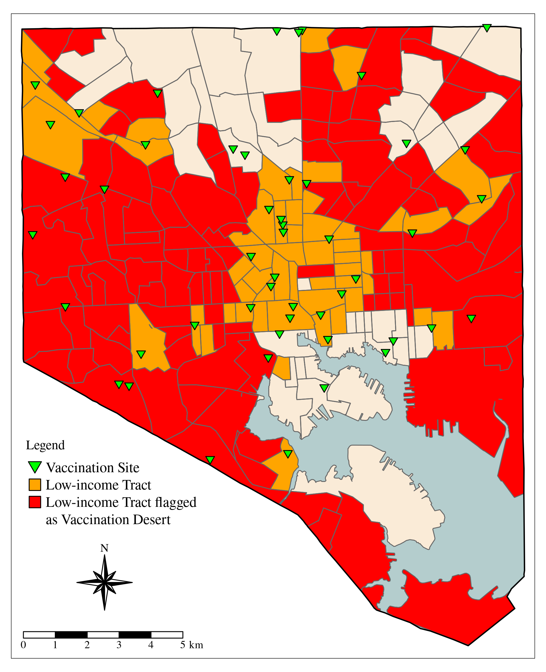
## 10 MULTIPOLYGON (((428077.1 18...Last, we map the potential vaccination deserts of Baltimore City. To make the map more appealing, we will clip the census tract map to the Baltimore City physical boundaries map.
BC_county_boundary <- subset(MD_counties_6487, COUNTY == "Baltimore City")

BC_county_boundary <- st_union(st_buffer(BC_county_boundary, dist = 20))

BC_CensusTracts_phys <- st_intersection(BC_CensusTracts, BC_county_boundary)

BC_LowIncome_phys <- st_intersection(BC_LowIncome, BC_county_boundary)

BC_VacDeserts_phys <- st_intersection(BC_VacDeserts, BC_county_boundary)

map_BC_phys <- tm_shape(BC) +
               tm_fill(col = "cornflowerblue") +
               tm_borders() +
               tm_shape(BC_CensusTracts_phys) +
               tm_fill(col = "antiquewhite") +
               tm_shape(BC_LowIncome_phys) +
               tm_fill(col = "orange") +
               tm_shape(BC_VacDeserts_phys) +
               tm_fill(col = "red") +
               tm_shape(BC_CensusTracts_phys) +
               tm_borders() +
               tm_shape(BC) +
               tm_borders(col = "black",
                          lwd = 1.5) +
               map_vac_BC +
#Legend
               tm_add_legend(type = "symbol",
                   labels =c('Vaccination Site',
                             'Low-income Tract',
                             'Low-income Tract flagged',
                             'as Vaccination Desert'),
                   size = c(0.5, 0.75, 0.75, 0),
                   shape = c(25, 22, 22, 20),
                   col = c('green', 'orange', 'red', 'white'),
                   title = 'Legend') +
               tm_layout(fontfamily = 'Times',
                   legend.position = c(0.025, 0.195),
                   legend.text.size = 0.75,
                   legend.width = 1) +
               tm_scale_bar(position = c("0.015", "0.0015"),
                            text.size = 0.55) + #add (default) scale
               tm_compass(type = "8star", size = 2.5,
                          position = c("0.1125", 0.07)) #add compass

map_BC_phys