Spatial Analysis and Mapping with R
5 Spatial Analysis—Part 1
This section introduces spatial analysis and mapping with R. It covers creation of spatial data, manipulation of spatial data, and mapping.
5.1 Creation and Manipulation of Spatial Data
Most manipulations are performed with functions from the sf package which is attached with the call library(sf).
library(sf)Conversion of non-spatial data into a (spatial) simple feature (sf) object
In Section 4.2 we created a smaller data frame of vaccination sites in Maryland (VaccineSites_mod). It is a non-spatial data frame that contains GPS coordinates in the variable Location. The format is (latitude, longitude).
str(VaccineSites_mod, strict.width = "cut")## 'data.frame': 556 obs. of 2 variables:
## $ name : chr "Luminis Health Anne Arundel Medical Center" "Luminis Health"..
## $ Location: chr "(38.990512076102, -76.5341664410021)" "(38.9825972406456, -"..Since the data frame has geometric information, it can be converted into a sf (simple feature) object with the function st_as_sf() from the sf package. sf objects contain non-spatial attributes (variables/columns) and spatial features (geometries) associated with the attributes (Pebesma & Bivand, 2021, Chapter 7). However, first we have to convert the geometric information into a format that sf can read.
st_as_sf() takes coordinates (in separate variables) and converts them into a single geometry (list) column. We therefore modify the Location variable, and split the variable into a lon and a lat variable that contain the longitude and latitude coordinates (as numbers), respectively.
# Copy VaccineSites_mod into new object
VaccineSites_mod2 <- VaccineSites_mod

# Remove round brackets
VaccineSites_mod2$Location <- gsub("[(]|[)]", "", VaccineSites_mod2$Location)

# Split columns
VaccineSites_mod2 <- tidyr::separate(VaccineSites_mod2, Location, c("lat", "lon"),
                                     sep = ", ", remove = TRUE, convert = TRUE)

str(VaccineSites_mod2, strict.width = "cut")
## 'data.frame': 556 obs. of 3 variables:
## $ name: chr "Luminis Health Anne Arundel Medical Center" "Luminis Health Doctors ...
## $ lon : num -76.5 -76.9 -76.6 -77 -76.9 ...The first line of the code copies the original data frame into a new object (VaccineSites_mod2). The next line removes the () from the entries in Location using a regex expression and the function gsub(). The regex identifies round brackets. gsub() substitutes the round brackets with no space (""). The 3rd line splits the variable into two variables (lat for latitude, and lon for longitude) with the function separate() from the package tidyr. The call tidyr::separate() allows to call the function separate() without attaching the package (tidyr). The original variable Location is removed (remove = TRUE), and the GPS coordinates are converted into real numbers (convert = TRUE).
Now we can use st_as_sf() to convert the coordinate variables into a single geometry column. GPS coordinates are based on the WGS 84 CRS (EPSG:4326), which is assigned to the geometries with the argument crs = 4326. Note, that coordinates in a sf geometry follow a lon, lat format.
VaccineSites_sf <- st_as_sf(VaccineSites_mod2,
                            coords = c("lon","lat"),
                            crs = 4326)
VaccineSites_sf
Changing Coordinate References Systems (Re-projection)
As mentioned in Section 2.3, spatial analyses involving distances require a projected coordinate reference system (CRS) with linear distance units (meter, US survey feet, etc.). For Maryland we use the NAD83(2011) Maryland CRS (EPSG:6487). It uses a Lambert Conformal Conic projection (lcc) and meters.
The function st_transform() from the sf package re-projects coordinates of simple feature objects.
VaccineSites_6487 <- st_transform(VaccineSites_sf, crs = 6487)

VaccineSites_6487
## Simple feature collection with 556 features and 1 field
## geometry type: POINT
## dimension: XY
## bbox: xmin: 192974.5 ymin: 37051.97 xmax: 564558.6 ymax: 228199.9
## projected CRS: NAD83(2011) / Maryland
## First 10 features:
## name
## 1 Luminis Health Anne Arundel Medical Center
## 2 Luminis Health Doctors Community Medical Center
## 3 Grace Medical Center (formerly Bon Secours Hospital)
## 4 Carroll Hospital Center
## 5 Howard County General Hospital
## 6 Holy Cross Hospital
## 7 MedStar Good Samaritan Hospital
## 8 MedStar Harbor Hospital
## 9 Greater Baltimore Medical Center
## 10 MedStar Southern Maryland Hospital Center
## geometry
## 1 POINT (440356.8 147055.9)
## 2 POINT (411663 146082.9)
## 3 POINT (430291.3 180062.2)
## 4 POINT (400805 209940)
## 5 POINT (409856.7 171801.7)
## 6 POINT (396836.2 149602.8)
## 7 POINT (435522.7 187900.9)
## 8 POINT (433214.1 176036.3)
## 9 POINT (432080.3 191488.2)
## 10 POINT (410811.8 120056.4)In Section 4.1 we already read in a map showing the boundaries of Maryland’s counties (MD_counties_map).
MD_counties_map## Simple feature collection with 24 features and 7 fields
## geometry type: MULTIPOLYGON
## dimension: XY
## bbox: xmin: -8848486 ymin: 4564403 xmax: -8354439 ymax: 4825752
## projected CRS: WGS 84 / Pseudo-Mercator
## First 10 features:
## OBJECTID COUNTY DISTRICT COUNTY_FIP COUNTYNUM CREATION_D LAST_UPDAT
## 1 1 Allegany 6 1 1 2010-01-28 2010-01-28
## 2 2 Anne Arundel 5 3 2 2006-04-18 2006-04-18
## 3 3 Baltimore 4 5 3 2006-10-09 2006-10-09
## 4 4 Baltimore City 0 510 24 2006-04-18 2009-11-16
## 5 5 Calvert 5 9 4 2010-01-28 2010-01-28
## 6 6 Caroline 2 11 5 2007-05-21 2008-07-30
## 7 7 Carroll 7 13 6 2008-06-16 2012-01-17
## 8 8 Cecil 2 15 7 2006-04-18 2008-08-20
## 9 9 Charles 5 17 8 2009-06-08 2009-06-08
## 10 10 Dorchester 1 19 9 2007-02-08 2007-02-22
## geometry
## 1 MULTIPOLYGON (((-8721085 48...
## 2 MULTIPOLYGON (((-8527741 47...
## 3 MULTIPOLYGON (((-8523507 48...
## 4 MULTIPOLYGON (((-8519244 47...
## 5 MULTIPOLYGON (((-8531762 46...
## 6 MULTIPOLYGON (((-8432189 47...
## 7 MULTIPOLYGON (((-8556981 47...
## 8 MULTIPOLYGON (((-8441053 48...
## 9 MULTIPOLYGON (((-8580309 46...
## 10 MULTIPOLYGON (((-8439760 46...The output tells us that the data set is using a projected CRS based on the WGS 84 CRS with a pseudo-mercator projection.
To map, all data objects need to have the same CRS. We therefore re-project the MD_counties_map to the NAD83(2011) Maryland CRS (EPSG:6487).
MD_counties_6487 <- st_transform(MD_counties_map, crs = 6487)

MD_counties_6487
## Simple feature collection with 24 features and 7 fields
## geometry type: MULTIPOLYGON
## dimension: XY
## bbox: xmin: 185218.2 ymin: 25771.53 xmax: 570274.7 ymax: 230947
## projected CRS: NAD83(2011) / Maryland
## First 10 features:
## OBJECTID COUNTY DISTRICT COUNTY_FIP COUNTYNUM CREATION_D LAST_UPDAT
## 1 1 Allegany 6 1 1 2010-01-28 2010-01-28
## 2 2 Anne Arundel 5 3 2 2006-04-18 2006-04-18
## 3 3 Baltimore 4 5 3 2006-10-09 2006-10-09
## 4 4 Baltimore City 0 510 24 2006-04-18 2009-11-16
## 5 5 Calvert 5 9 4 2010-01-28 2010-01-28
## 6 6 Caroline 2 11 5 2007-05-21 2008-07-30
## 7 7 Carroll 7 13 6 2008-06-16 2012-01-17
## 8 8 Cecil 2 15 7 2006-04-18 2008-08-20
## 9 9 Charles 5 17 8 2009-06-08 2009-06-08
## 10 10 Dorchester 1 19 9 2007-02-08 2007-02-22
## geometry
## 1 MULTIPOLYGON (((284864.2 22...
## 2 MULTIPOLYGON (((434019 1735...
## 3 MULTIPOLYGON (((437063.4 22...
## 4 MULTIPOLYGON (((440528 1894...
## 5 MULTIPOLYGON (((431100.8 12...
## 6 MULTIPOLYGON (((508262.9 16...
## 7 MULTIPOLYGON (((411297.8 20...
## 8 MULTIPOLYGON (((500588 2260...
## 9 MULTIPOLYGON (((393194.3 11...
## 10 MULTIPOLYGON (((503022.8 11...5.2 First Maps
Lets plot the vaccination sites onto a map of Maryland counties using tmap. tmap is a R package designed to create thematic maps to visualize spatial distributions. It uses a layer based approach. Every map starts with tm_shape(). tm_shape() defines the extension of the map and which method can be used to draw the features. It is followed by other layer elements, such as tm_fill() (which colors polygons), tm_borders() (which outlines polygons), or tm_symbols() (which plots markers and symbols), to name a few (Lovelace et al., 2021, Chapter 8). Each layer can be stored in or assigned to an object that can be called separately.
Mapping Vaccination Sites
To start, we create a “base map” of Maryland’s counties that is stored in the object map_MD_counties. tm_shape() is called to create a layer based on the shape object MD_counties_6487. tm_polygon() plots the polygons defined in MD_counties_6487. We could use the argument "MAP_COLORS" to color the counties as it attempts to color the polygons in such a way that neighboring polygons have different colors. However, it does not work too well for our data set. Furthermore, its color attribution is not consistent. Therefore, we will define our own color scheme that is based on the color palette GnBu from the RColorBrewer package.
library(tmap)
library(RColorBrewer)

#Define colors
(cols <- brewer.pal(brewer.pal.info["GnBu", "maxcolors"], "GnBu"))

mypal <- c(cols[1], cols[4], cols[3], cols[5], cols[3],
           cols[1], cols[4], cols[4], cols[5], cols[4],
           cols[2], cols[2], cols[1], cols[5], cols[5],
           cols[3], cols[1], cols[3], cols[1], cols[4],
           cols[5], cols[4], cols[3], cols[4])

# map counties
map_MD_counties <- tm_shape(MD_counties_6487) +
          tm_polygons(col = "COUNTY",
          palette = mypal,
          legend.show = FALSE)

map_MD_counties
map_MD_counties plots the map and you should see a plot similar to Fig. 5.1 A.
Create a directory figures in your project directory. Save the map of the county with tmap_save() as a .png file (map_MD_counties.png) in the directory figures (within the current working directory):
# save to png
tmap_save(map_MD_counties, filename = "figures/map_MD_counties.png")
Then we create a layer that has the labels of the counties. The layer is assigned to the object MD_counties_label. Again, tm_shape(MD_counties_6487) is called. tm_text plots the name of the counties (listed in the variable COUNTY of the MD_counties_6487 data set). We set the text color to brown (argument col), and the size to 0.75. We plot the labels by calling the object MD_counties_label. A plot similar to Fig. 5.1 B should be produced.
#label
MD_counties_label <- tm_shape(MD_counties_6487) +
                     tm_text("COUNTY",
                             col = "brown",
                             size = 0.75)
MD_counties_label
Last, we create a layer with the vaccination sites and store the layer in the object map_VaccineSites. tm_shape() is called again to create the layer based on the VaccineSites_6487 object. The geometric features of this layer are points. The points are plotted with the function tm_symbols(). The shape argument plots symbols available to R (shape 0 to 25). The fill color, outline (border) color, and line width of the outline of shapes 21 to 25 can be changed with the arguments col, border.col, and border.lwd, respectively (Figure 5.1 D). For the vaccine sites (Figures 5.1 C, 5.2, and 5.3) the fill color is set to green, the outline color to red, and the line width to 1. Calling map_VaccineSites should plot a plot similar to Figure 5.1 C.
# map vaccine sites
map_VaccineSites <- tm_shape(VaccineSites_6487) +
          tm_symbols(shape = 25,
                     size =0.3,
                     col = "green",
                     border.col = "red",
                     border.lwd = 1)
map_VaccineSites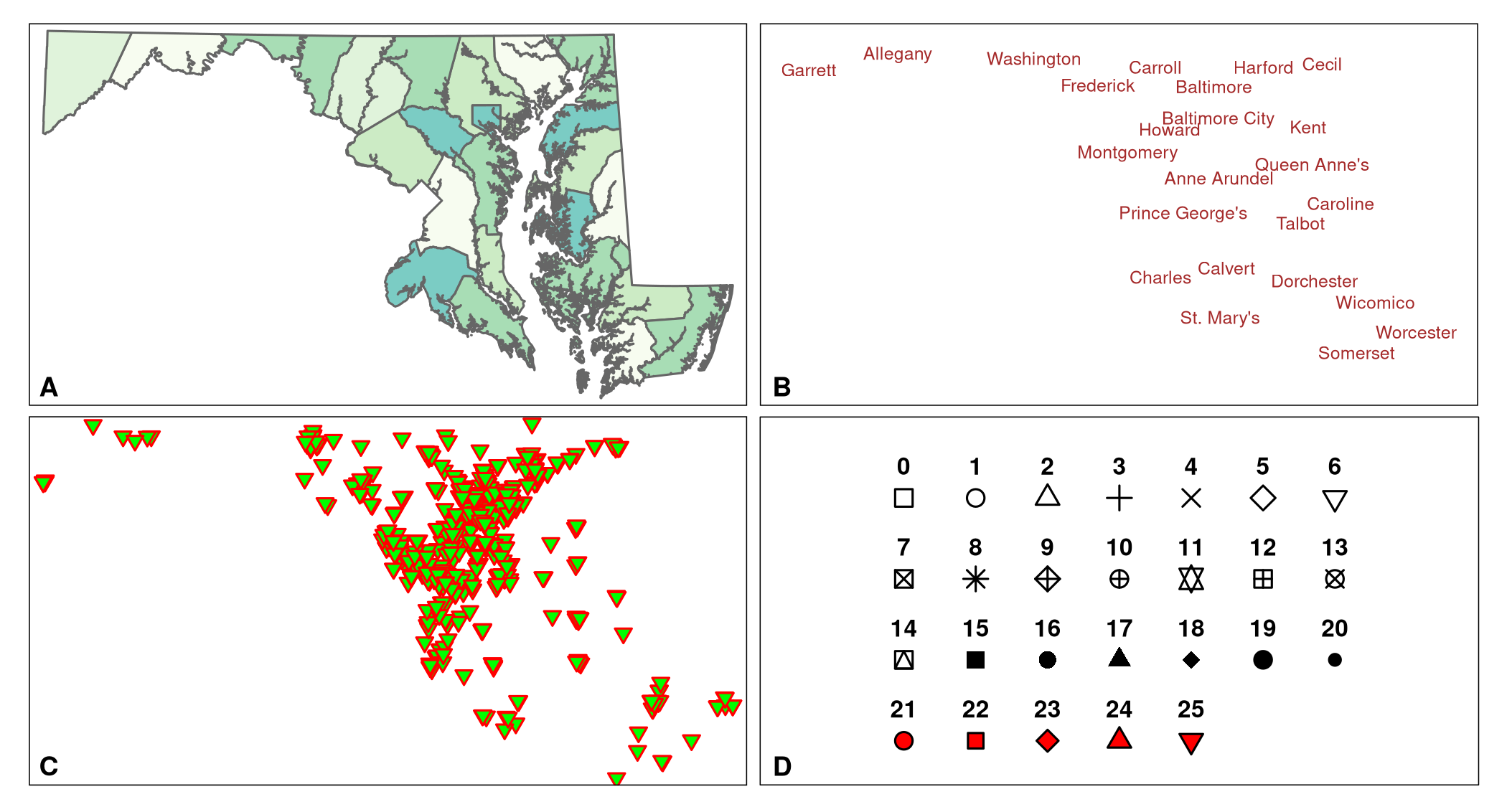
R.We can put together the final map by calling the layers, and add a legend with tmap_add_label().
MD_vac1 <- map_MD_counties +
           MD_counties_label +
           map_VaccineSites +
           tm_add_legend(type = "symbol",
                         shape = 25,
                         size = 0.75,
                         col = "green",
                         border.col = "red",
                         label = "COVID-19 Vaccination Site") +
            tm_layout(legend.text.size = 1)
MD_vac1
tm_add_legends() adds (manually) a legend to the plot. We just want to indicate what the plotted symbols stand for (i.e, COVID-19 Vaccination Sites). Therefore, the type is set to "symbol." We define the shape, fill and outline color (copy the respective parameters (arguments) from tm_symbols), and the size of the symbol for the legend. label adds the legend text ("COVID-19 Vaccination Site"). The last function, tm_layout() allows to fine tune the plot. Here we only specify the size of the legend label. The last line (MD_vac1) plots the map. The plot should look similar to the plot in Figure 5.2.
Save the plot as a .png file (MD_vac_sites.png) in the directory figures (within the current working directory).
# save to png
tmap_save(MD_vac1, filename = "figures/MD_vac_sites.png")
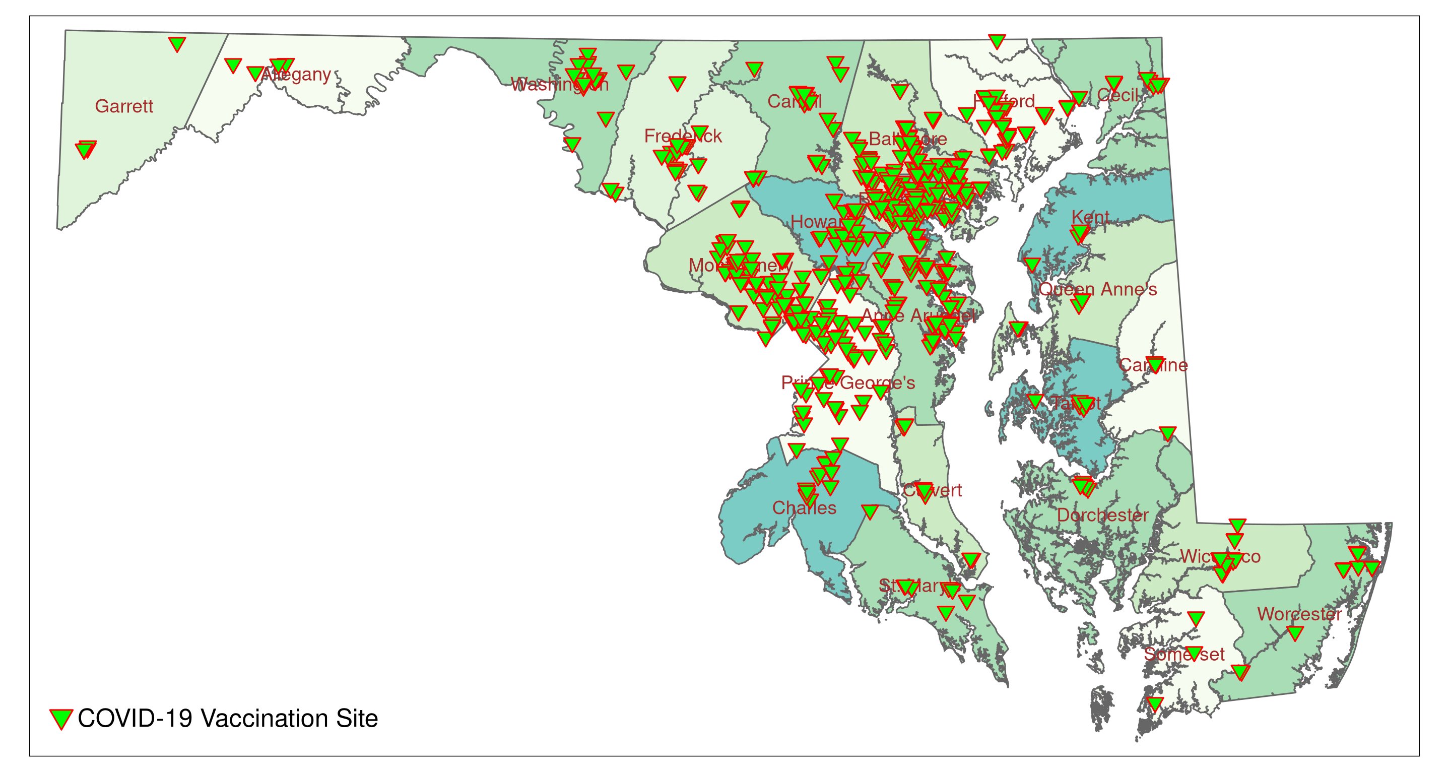
The map shows that there are clusters of vaccination sites in the I-95 and I-270 corridors. Rural areas seem to be less covered. To check we can add urban census tracts to the plot. The data frame MD_CensusTracts_Map has all the information we need. However, its CRS is NAD83.
MD_CensusTracts_Map ## Simple feature collection with 1403 features and 13 fields
## geometry type: MULTIPOLYGON
## dimension: XY
## bbox: xmin: -79.48765 ymin: 37.91172 xmax: -75.04894 ymax: 39.72304
## geographic CRS: NAD83
## First 10 features:
## CensusTract GEO_ID STATE COUNTY TRACT NAME LSAD CENSUSAREA
## 1 24001000100 1400000US24001000100 24 001 000100 1 Tract 187.937
## 2 24001000200 1400000US24001000200 24 001 000200 2 Tract 48.067
## 3 24001000300 1400000US24001000300 24 001 000300 3 Tract 8.656
## 4 24001000400 1400000US24001000400 24 001 000400 4 Tract 3.723
## 5 24001000500 1400000US24001000500 24 001 000500 5 Tract 4.422
## 6 24001000600 1400000US24001000600 24 001 000600 6 Tract 1.577
## 7 24001000700 1400000US24001000700 24 001 000700 7 Tract 0.712
## 8 24001000800 1400000US24001000800 24 001 000800 8 Tract 1.255
## 9 24001001000 1400000US24001001000 24 001 001000 10 Tract 0.448
## 10 24001001100 1400000US24001001100 24 001 001100 11 Tract 0.301
## County Urban POP2010 LowIncomeTracts HUNVFlag
## 1 Allegany 0 3718 1 0
## 2 Allegany 0 4564 1 0
## 3 Allegany 0 2780 1 0
## 4 Allegany 1 3022 1 0
## 5 Allegany 1 2734 1 0
## 6 Allegany 1 2965 1 0
## 7 Allegany 1 3387 1 1
## 8 Allegany 1 2213 1 1
## 9 Allegany 1 2547 1 0
## 10 Allegany 1 1493 1 0
## geometry
## 1 MULTIPOLYGON (((-78.42058 3...
## 2 MULTIPOLYGON (((-78.71775 3...
## 3 MULTIPOLYGON (((-78.72077 3...
## 4 MULTIPOLYGON (((-78.70206 3...
## 5 MULTIPOLYGON (((-78.75435 3...
## 6 MULTIPOLYGON (((-78.74107 3...
## 7 MULTIPOLYGON (((-78.75033 3...
## 8 MULTIPOLYGON (((-78.76588 3...
## 9 MULTIPOLYGON (((-78.77711 3...
## 10 MULTIPOLYGON (((-78.76443 3...We re-project MD_CensusTracts_Map to NAD83(2011) Maryland (EPSG:6487).
MD_CensusTracts_6487 <- st_transform(MD_CensusTracts_Map, crs = 6487)
MD_CensusTracts_6487
## Simple feature collection with 1403 features and 13 fields
## geometry type: MULTIPOLYGON
## dimension: XY
## bbox: xmin: 185230.9 ymin: 27801.06 xmax: 570294.2 ymax: 230941.9
## projected CRS: NAD83(2011) / Maryland
## First 10 features:
## CensusTract GEO_ID STATE COUNTY TRACT NAME LSAD CENSUSAREA
## 1 24001000100 1400000US24001000100 24 001 000100 1 Tract 187.937
## 2 24001000200 1400000US24001000200 24 001 000200 2 Tract 48.067
## 3 24001000300 1400000US24001000300 24 001 000300 3 Tract 8.656
## 4 24001000400 1400000US24001000400 24 001 000400 4 Tract 3.723
## 5 24001000500 1400000US24001000500 24 001 000500 5 Tract 4.422
## 6 24001000600 1400000US24001000600 24 001 000600 6 Tract 1.577
## 7 24001000700 1400000US24001000700 24 001 000700 7 Tract 0.712
## 8 24001000800 1400000US24001000800 24 001 000800 8 Tract 1.255
## 9 24001001000 1400000US24001001000 24 001 001000 10 Tract 0.448
## 10 24001001100 1400000US24001001100 24 001 001100 11 Tract 0.301
## County Urban POP2010 LowIncomeTracts HUNVFlag
## 1 Allegany 0 3718 1 0
## 2 Allegany 0 4564 1 0
## 3 Allegany 0 2780 1 0
## 4 Allegany 1 3022 1 0
## 5 Allegany 1 2734 1 0
## 6 Allegany 1 2965 1 0
## 7 Allegany 1 3387 1 1
## 8 Allegany 1 2213 1 1
## 9 Allegany 1 2547 1 0
## 10 Allegany 1 1493 1 0
## geometry
## 1 MULTIPOLYGON (((277992.7 21...
## 2 MULTIPOLYGON (((252677.1 22...
## 3 MULTIPOLYGON (((252464.7 22...
## 4 MULTIPOLYGON (((253978.3 22...
## 5 MULTIPOLYGON (((249423 2212...
## 6 MULTIPOLYGON (((250523.8 21...
## 7 MULTIPOLYGON (((249749.1 22...
## 8 MULTIPOLYGON (((248425.6 22...
## 9 MULTIPOLYGON (((247506.5 22...
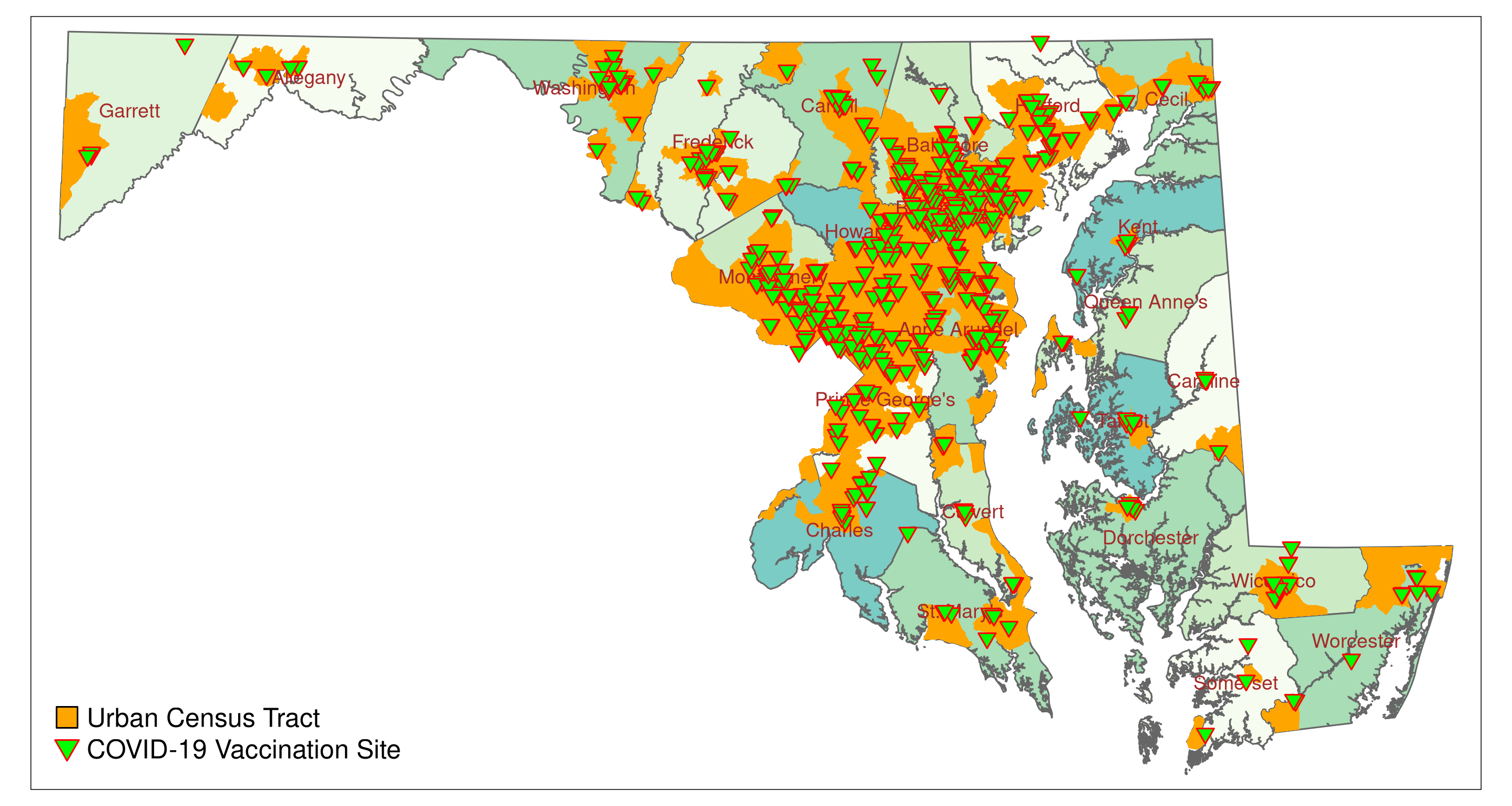
## 10 MULTIPOLYGON (((248561.4 22...For the map we are only interested in urban census tracts. We extract the urban tracts from MD_CensusTracts_6487 (Urban == 1), and re-draw the map. Urban tracts are highlighted in orange.
# Filter out urban centers
urban_tracts <- subset(MD_CensusTracts_6487, Urban == 1)

urban_tracts

# Map urban tracts
# Layer for urban tracts
map_urban_tracts <- tm_shape(urban_tracts) +
                    tm_fill(col = "orange")

# save as png
tmap_save(map_urban_tracts, filename = "figures/map_urban_tracts.png")
Compile the map.
MD_vac2 <- map_MD_counties +
           map_urban_tracts +
           MD_counties_label +
           map_VaccineSites +
           tm_add_legend(type = "symbol",
                         shape = c(22, 25),
                         size = c(1, 0.75),
                         col = c("orange", "green"),
                         border.col = c("black", "red"),
                         label = c("Urban Census Tract",
                                   "COVID-19 Vaccination Site")) +
           tm_layout(legend.text.size = 1)

MD_vac2

# save to png
tmap_save(MD_vac2, filename = "figures/MD_vac2_sites_census_tract.png")
We added an orange square (symbol 22) in tm_add_legend():
           tm_add_legend(type = "symbol",
                         shape = c(22, 25),
                         size = c(1, 0.75),
                         col = c("orange", "green"),
                         border.col = c("black", "red"),
                         label = c("Urban Census Tract", "COVID-19 Vaccination Site"))
Calling Map_vac2 should produce a plot similar to Figure 5.3.
5.3 Manipulating Geometries
The sf package has functions that allow us to manipulate the spatial features of a sf object, including
- identify features based on their spatial relation to other features,
- clip geometries, and
- merge geometries.
Identify spatial features based on spatial relations to other features
To identify or visualize vaccination sites in rural and urban centers, we plotted urban tracts onto the vaccination site map. Alternatively, we can extract vaccination sites that are located in rural tracts and urban centers with the function st_intersection().
We already created a sf object that features urban census tracts (urban_tracts). Lets also create a sf object for rural census tracts.
rural_tracts <- subset(MD_CensusTracts_6487, Urban == 0)The following lines of code identify the vaccination sites that are located within or on the border of urban and rural census tracts, respectively. You will likely see warnings. They can be ignored.
vac_urban <- st_intersection(urban_tracts, VaccineSites_6487)## Warning: attribute variables are assumed to be spatially constant throughout all
## geometriesvac_urban## Simple feature collection with 494 features and 14 fields
## geometry type: POINT
## dimension: XY
## bbox: xmin: 192974.5 ymin: 46073.83 xmax: 560461.9 ymax: 224285.4
## projected CRS: NAD83(2011) / Maryland
## First 10 features:
## CensusTract GEO_ID STATE COUNTY TRACT NAME LSAD
## 40 24003702701 1400000US24003702701 24 003 702701 7027.01 Tract
## 1070 24033806711 1400000US24033806711 24 033 806711 8067.11 Tract
## 1301 24510200100 1400000US24510200100 24 510 200100 2001 Tract
## 394 24013507801 1400000US24013507801 24 013 507801 5078.01 Tract
## 629 24027605602 1400000US24027605602 24 027 605602 6056.02 Tract
## 829 24031703901 1400000US24031703901 24 031 703901 7039.01 Tract
## 1369 24510270803 1400000US24510270803 24 510 270803 2708.03 Tract
## 1323 24510250203 1400000US24510250203 24 510 250203 2502.03 Tract
## 314 24005490605 1400000US24005490605 24 005 490605 4906.05 Tract
## 926 24033801207 1400000US24033801207 24 033 801207 8012.07 Tract
## CENSUSAREA County Urban POP2010 LowIncomeTracts HUNVFlag
## 40 1.812 Anne Arundel 1 4815 0 0
## 1070 0.548 Prince George's 1 5146 1 0
## 1301 0.102 Baltimore City 1 1846 1 1
## 394 2.423 Carroll 1 5652 0 1
## 629 2.809 Howard 1 7610 0 0
## 829 0.554 Montgomery 1 2957 0 0
## 1369 0.845 Baltimore City 1 6268 1 0
## 1323 0.357 Baltimore City 1 2018 1 1
## 314 0.844 Baltimore 1 5182 1 0
## 926 3.141 Prince George's 1 4432 0 0
## name
## 40 Luminis Health Anne Arundel Medical Center
## 1070 Luminis Health Doctors Community Medical Center
## 1301 Grace Medical Center (formerly Bon Secours Hospital)
## 394 Carroll Hospital Center
## 629 Howard County General Hospital
## 829 Holy Cross Hospital
## 1369 MedStar Good Samaritan Hospital
## 1323 MedStar Harbor Hospital
## 314 Greater Baltimore Medical Center
## 926 MedStar Southern Maryland Hospital Center
## geometry
## 40 POINT (440356.8 147055.9)
## 1070 POINT (411663 146082.9)
## 1301 POINT (430291.3 180062.2)
## 394 POINT (400805 209940)
## 629 POINT (409856.7 171801.7)
## 829 POINT (396836.2 149602.8)
## 1369 POINT (435522.7 187900.9)
## 1323 POINT (433214.1 176036.3)
## 314 POINT (432080.3 191488.2)
## 926 POINT (410811.8 120056.4)vac_rural <- st_intersection(rural_tracts, VaccineSites_6487)## Warning: attribute variables are assumed to be spatially constant throughout all
## geometriesvac_rural## Simple feature collection with 62 features and 14 fields
## geometry type: POINT
## dimension: XY
## bbox: xmin: 219869 ymin: 37051.97 xmax: 564558.6 ymax: 228199.9
## projected CRS: NAD83(2011) / Maryland
## First 10 features:
## CensusTract GEO_ID STATE COUNTY TRACT NAME LSAD
## 353 24009860702 1400000US24009860702 24 009 860702 8607.02 Tract
## 1091 24035810400 1400000US24035810400 24 035 810400 8104 Tract
## 1106 24037875500 1400000US24037875500 24 037 875500 8755 Tract
## 1120 24039930300 1400000US24039930300 24 039 930300 9303 Tract
## 1198 24047951300 1400000US24047951300 24 047 951300 9513 Tract
## 366 24011955301 1400000US24011955301 24 011 955301 9553.01 Tract
## 465 24019970702 1400000US24019970702 24 019 970702 9707.02 Tract
## 1129 24041960501 1400000US24041960501 24 041 960501 9605.01 Tract
## 1185 24045010702 1400000US24045010702 24 045 010702 107.02 Tract
## 1194 24047950900 1400000US24047950900 24 047 950900 9509 Tract
## CENSUSAREA County Urban POP2010 LowIncomeTracts HUNVFlag
## 353 9.430 Calvert 0 2974 1 0
## 1091 47.327 Queen Anne's 0 6053 0 0
## 1106 34.068 St. Mary's 0 8631 0 1
## 1120 88.028 Somerset 0 2539 1 0
## 1198 5.936 Worcester 0 2816 1 0
## 366 42.331 Caroline 0 4111 0 0
## 465 43.137 Dorchester 0 3987 0 0
## 1129 22.790 Talbot 0 4752 0 0
## 1185 27.469 Wicomico 0 8671 1 1
## 1194 26.689 Worcester 0 2017 0 0
## name geometry
## 353 Calvert County Health Department POINT (435102 99044.7)
## 1091 Queen Anne's County Health Department POINT (481028.7 153466.8)
## 1106 Saint Mary's County Health Department POINT (431747.9 70311.09)
## 1120 Somerset County Health Department POINT (513236.4 51719.08)
## 1198 Worcester County Health Department POINT (542330.9 57518.24)
## 366 Walmart Denton POINT (502252.9 134723)
## 465 Walmart Cambridge POINT (482594.3 98828.14)
## 1129 Walmart Easton POINT (482184.2 123210.8)
## 1185 Walmart Salisbury POINT (524947.9 84315.16)
## 1194 Walmart Berlin POINT (560573.2 76351.68)Sixty-two vaccination sites are in rural tracts, and 494 in urban tracts. Let’s see how many vaccination sites per 100,000 (or in scientific notation 1e05) residents are in rural and urban tracts (based on population data from the 2010 census). The variable POP2010 lists the total number of residents in each tract. The number of vaccination sites for each subset equals the number of entries and can be displayed with nrow(). nrow() lists the number of rows of a data frame.
rural_pop_100k <- nrow(vac_rural)/sum(vac_rural$POP2010)*1e05
rural_pop_100k
## [1] 21.07353urban_pop_100k <- nrow(vac_urban)/sum(vac_urban$POP2010)*1e05
urban_pop_100k## [1] 21.07604The result suggests that based on the plain number of vaccination sites, rural and urban tracts are overall equally covered. Rural tracts have 21.07 vaccination sites per 100,000 residents, and urban tracts 21.08.
To visualize, we map the urban and rural vaccination sites (green inverted triangles (symbol 25): urban, blue diamonds (symbol 23): rural sites; for symbols, see Figure 5.1 D). We compile the map as we have done before. First, we create map layers for the urban and rural vaccination sites. Then we add these two layers to the county map featuring urban tracts.
map_vac_urban <- tm_shape(vac_urban) +
                 tm_symbols(shape = 25,
                            size =0.3,
                            col = "green",
                            border.col = "red",
                            border.lwd = 1)

map_vac_rural <- tm_shape(vac_rural) +
                 tm_symbols(shape = 23,
                            size =0.3,
                            col = "blue",
                            border.col = "red",
                            border.lwd = 1)

MD_vac3 <- map_MD_counties +
           map_urban_tracts +
           MD_counties_label +
           map_vac_urban +
           map_vac_rural +
           tm_add_legend(type = "symbol",
                         shape = c(22, 25, 23),
                         size = c(1, 0.75, 0.75),
                         col = c("orange", "green", "blue"),
                         border.col = c("black", "red", "red"),
                         label = c("Urban Census Tract",
                                   "Urban COVID-19 Vaccination Site",
                                   "Rural COVID-19 Vaccination Site")) +
           tm_layout(legend.text.size = 1)

#call map
MD_vac3

# save to png
tmap_save(MD_vac3, filename = "figures/MD_vac3_urban_rural.png")
The code should print a map similar to Figure 5.4.

References
Lovelace, R., Nowosad, J., & Jannes, M. (2021). Geocomputation with R. https://geocompr.robinlovelace.net/ index.html
Pebesma, E., & Bivand, R. (2021). Spatial data science with applications in R. https://keen-swartz-3146c4.netlify.app/index.html
