Chapter 3. Significance Tests and Assumptions

Jiwon N. Speers

Chapter 3. Significance Tests and Assumptions

I. Significance Tests

We want to test whether the relationships that we see in the sample exist in the population. Note this expression implies inferential statistics. If the null hypothesis about the slope is rejected (in other words, if the p-value is smaller than .05), then we will interpret either $b_1$ or the standardized slope $b_1*$ to determine whether a statistically significant (non-zero) value is large enough (to be substantively important). In other words, if the p-value is not smaller than .05, then we don’t need to interpret $b_1$ or the beta weight $b_1*$ .

Also when doing hypothesis tests, some conditions (the so-called “assumptions”) will need to be checked in advance, so we can assess whether our test results are believable.

The simplest hypothesis test using r tests whether the correlation is zero in the population ( $=H_0$ ). That is, we want to determine the probability that an observed $r$ (= sample statistic) came from a hypothetical null parameter ( $H_0: \rho = 0$ ). In other words, the null hypothesis is the correlation is 0 in the population.

Sometimes this t statistic is squared, which results in an F statistic with 1 and n – 2 degrees of freedom (the p-value is the same, regardless of which test is used).

Returning to [Exercise 1], wages and factory workers’ productivity example (see Chapter 1), our r was .65. We can test the null hypothesis that the correlation came from a population in which wages and workers’ productivity are unrelated (where $\rho = 0$ ).

We can compare the t value to a critical value in a t table or look up the p-value using SPSS or Excel. The .05 critical value for $df = n - 2 = 28$ is 2.048. This is when we have only one $X$ variable in the model.

From $b = r \times \frac{S_y}{S_x}$ ,

$b_1* = r_{xy}$ for the equation $Z(Y_i) = {b_1}^* Z(X_i) + {e_i}^*$ is derived.

Since the sample t = 4.53 and the critical value is 2.048, our sample t is greater than the critical t (let us call it $t_c$ ) and so we reject the null hypothesis that $\rho = 0$ . Also with $df = n - 2 = 28$ , the p-value for this statistic is just about .0001. Using Excel we can enter the Excel function “tdist” to get the p-value:

tdist(4.53, 23, 2) = .0001001
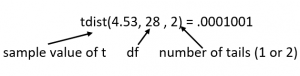
Since we reject the null hypothesis, we conclude that there is a non-zero correlation between wages and workers’ productivity in the population. The $r = .65$ and the squared correlation equals .43, which indicates (based on Cohen’s rules of thumb) that the effect is large.

The test of the null hypothesis that $\rho = 0$ is the same as the test of the null hypothesis that $\beta_1= 0$ (i.e., the parameter estimated by the slope, $b_1$ , is 0), when we have a regression based on only one $X$ . (With more $X$ this is not the case.)

If there is no relationship between $X$ and $Y$ , then the correlation $\rho$ equals zero. This is the same thing as the slope of the regression line $\beta_1$ equaling zero, where the line is flat. This flat line also represents a situation where the mean of $Y$ is the best and only predicted value ( $\hat{Y} = \bar{Y}$ for all cases) and the standard error of the estimate (SEE) will be very close to the standard deviation of $Y$ .

What are SEE? SEE is the SD of the residuals (the $e_i$ ) around the line, also called the root mean squared error. It can be computed in several ways and you do not need to memorize these formulas. Using $n$ , $e^2$ , $MSE$ and $p$ (the number of predictors) as

$SEE = \sqrt{MSE} = \sqrt{\Sigma {e_i}^2 / (n - p - 1)}$

Recall that the t-test typically compares an observed parameter to a hypothetical (null) value, dividing the difference by the standard error. The test for $r$ was formed in that way (as is the two-sample t for mean differences). Our t-test is $t = (b_1 - \beta_1) / S_{b1}$ .

Here, for a test of $\beta_1$ we need a standard error (SE) for $b_1$ . It is

$S_{b1} = \frac{SEE}{S_X \sqrt{n - 1}} = \frac{SEE}{\sqrt{\Sigma{(X_i - \bar{X})}^2}} = \frac{SEE}{\sqrt{SSX}}$

SSX is shorthand for the “Sum of Squares of $X$ ” which is part of the variance of $X$ . The greater the variance of $X$ values in your data, the larger SSX will be.

$SSX = \Sigma{(X_i - \bar{X})}^2$

Now let us consider the formula for the SE of the slope ( $S_{b1}$ ).

$S_{b1}$ gets smaller when

SEE gets small – this is the standard deviation of the regression residuals. Better “fit” means smaller SEE and smaller $S_{b1}$
$S_x$ gets large – this means we are seeing a larger range of $X$ values and that is good – it helps us get a better sense of the value of $b_1$
$n$ gets large – more data gives us more precision

Recall what the SE of the slope represents.

$S_{b1}$ is the estimated value of the standard deviation of a hypothetical large set of slopes. (Recall that the SE of the mean of $Y$ is $S_Y / {\sqrt{n}$ ).
$S_{b1}$ is the SD we would get if we sampled repeatedly from the population of interest, and computed a large collection of slopes ( $b_1s$ ) that estimate the same slope $b_1$ .
So we would like $S_{b1}$ to be small because it means we have a precise estimate of $b_1$ in our sample.

Let us return to the test. The t-test for comparing $b_1$ to a null parameter (typically $b_1 = 0$ ) is a t-test with $n - 2$ , $df$ .

$t = \frac{b_1 - \beta_1}{S_{b_1}} = \frac{b_1}{SEE / S_X\sqrt{n-1}} = \frac{b_1S_x\sqrt{n-1}}{SEE}$

Similarly, we can create a confidence interval (CI) around the observed $b_1$ using the following extension of the t-test formula.

$95\%CI(\beta_1) = b_1\pm t_{\alpha / 2} (\frac{SEE}{S_X\sqrt{n-1}}) = b_1\pm t_{\alpha / 2}S_{b1}$

If the CI does not capture 0, we would then reject the null hypothesis that our $b_1$ came from a population with $\beta_1 = 0$

Learning Check

Indicators of model quality:
- MSE (compared to ${S^2}_Y$ ), SEE (compared to $S_Y$ )
- $R^2$ (want it close to 1) or also $r$ (should be close to -1 or 1)
- $b_1$ and ${b^*}_1$ (want both to be large) only for simple regression (Since we learn the steps of regression in the section of simple regression, the slope coefficients were placed here; however, they are originally the indicators for an individual slope.)
Tests:
- F test for model F= MSR/MSE
  - $H_0: \rho^2 = 0$ (or $H_0: \beta_1 = 0$ if it is a simple regression)
- t test for slope
  - $H_0: \beta_1 = 0$
Interval estimate:
- The CI for
  - $b_1 \pm t S_{b1}$

[Exercise 5]

For the wages and workers’ productivity data, the standard error of is computed below.

$b_1 = .00455$

$SEE = .54$

$S_X = 100$

(1) If we had 30 participants, how would you compute S_b1and t statistic? Use the following formulas.

$S_{b_1} = \frac{SEE}{S_X\sqrt{n-1}}$

$t = \frac{b_1}{S_{b_1}}$

(2) The two-tailed critical t for $\alpha = .05$ with 28 degrees of freedom equals 2.05, so how would you compute the CI? Compute the upper limit (UL) and lower limit (LL). Fill in the blanks.

$95\%CI(\beta_1) = b_1 \pm t_{\alpha / 2}S_{b_1} =$ ( ) $\pm$ 2.05 $\times$ ( )

$UL =$

$LL =$

(3) Based on the above (2), since 0 does not fall between the LL and the UL, would we reject or not reject the null hypothesis that our $b_1$ came from a population with $\beta_1 = 0$ ?

II. Assumptions in Regression

We will learn about the assumptions needed for doing hypothesis tests. These assumptions involve the residuals from the model, so we need to estimate a model before we can check assumptions. So, we will do some analyses of residuals, and eventually (for multiple regression) we will look for multicollinearity.

In order for our tests to work properly (that is, to reject the null hypotheses the correct portion of the time, etc.) we need to make some assumptions.

1. Assumptions for Tests of $\rho$ and $\beta_1$ : Linearity

For both correlation and regression, we assume that the relationship between $X$ and $Y$ is linear rather than curvilinear. Different procedures are available for modeling curvilinear data. We can check this assumption by looking at the X-Y scatterplot.

2. Assumptions for Tests of $\rho$ and $\beta_1$ : Independence

Another assumption of both regression and correlation is that the data pairs are independent of each other. We do not assume $X$ is independent of $Y$ , but rather that ( $X_1$ , $Y_1$ ) is independent of ( $X_2$ , $Y_2$ ) and ( $X_3$ , $Y_3$ ) etc.—in general we assume that ( $X_i$ , $Y_i$ ) for any case $i$ is independent of ( $X_j$ , $Y_j$ ) for another case $j$ .

This means, for example, we do not want to have subgroups of cases that are related—so e.g., if the data are scores on, say, $X$ = length of the marriage and $Y$ = marital satisfaction, we don’t want scores for a sample including husbands and wives who are married to each other.

Unfortunately, there is no statistical or visual test for independence. We simply need to understand the structure of the data. We can find out about independence by knowing how the data were collected. So for instance in the example, I gave, if we knew that only one member of any married couple provided data on $X$ = length of the marriage and $Y$ = marital satisfaction, we might consider the cases to be independent.

Can you think of things that might cause scores on $X$ and $Y$ not to be independent even if data were collected from people not married to each other?

3. Assumptions for Correlation: Bivariate Normality

To draw inferences about the correlation coefficient, we need to make only one assumption in addition to linearity and independence (albeit a rather demanding assumption).

If we wish to test hypotheses about $\rho$ or establish confidence limits on $\rho$ , we must assume that the joint distribution of $X$ and $Y$ is normal. We check this by inspecting the X-Y scatterplot.

Graph of joint distribution analysis

4. Assumptions for Regression:

Also, if we wish to draw inferences about regression parameters (e.g., create CIs around $b_1$ or $\hat{Y}$ or test a hypothesis about the value of $\beta_1$ ), we need to make more assumptions:

(1) Homogeneity of variances: The error variances are equal across all levels of $X$ . The observed variances do not need to be identical, but it is necessary that they could have reasonably come from a common population parameter. If the variances are unequal, then SEE (for which we estimate a single value) is not a valid descriptive statistic for all conditional error distributions (conditional on the value of $X$ ).

Usually, we check the homogeneity of error variances by examining error plots (i.e., residual scatter plots). Only if we have a great amount of data can we examine error-variance values at different values of $X$ . One typical plot is a scatter plot of $X$ or $\hat{Y}$ on the horizontal axis and the residuals or even standardized residuals on the vertical axis. We look for a similar spread of points at each place along the horizontal axis. In other words, we are looking for a cloud of points and to see equal spread vertically. We want to be sure we do not see odd patterns in the data. In other words, we do not want to see a fan shape (e.g., more spread for high $X$ than low $X$ ) or a curvilinear pattern, which suggests something may be missing from the model.

(2) Normality: The distribution of observed $Y$ around predicted $Y$ ( $\hat{Y}$ ) at each value of $X$ (the so-called conditional distributions) are assumed to be normal in shape. This is necessary because we use the normal distribution to lead to the hypothesis tests we do. What we look at here is the normality of the residuals. To check the normality of the residuals we ask for a histogram of the residuals when we run the regression.

(3) Model specification. We need to make the big assumption that the model is “properly specified.” This can be broken into a few pieces:

- All important $X$ are in the model: Frankly, for the simple regression (just one $X$ ) this assumption is most often not true. Can you think of any outcome where only one thing predicts it? Also, some people consider the assumption about linearity to be part of this larger assumption – that is, we can have $X$ in the model but if it is not linearly related to $Y$ the model may still not be properly specified (e.g., we may need $X^2$ in the model).
- No useless $X$ are in the model: This part of the assumption says no predictors that are unrelated to $Y$ are in the model. For the simple regression, this is not really applicable – it will come up when we have several $X$ in the model (i.e., for multiple regression).

As was true for independence there is no single test for model specification. We can evaluate the two parts of the assumption using logic and (eventually) tests of the model. For now, we can only assess the first part, and we can pretty much assume it is false when we have only one $X$ . A part of the rationale here is simply to look at the literature in any area and see what the important predictors of your $Y$ have been discovered to be, to date. One way to suggest this assumption is wrong is to find at least one predictor (other than the one in your model) that relates significantly to $Y$ .

When we examine multiple regression models we will see how to assess the second part, by deciding whether there are “useless $X$ ” in the model.

Meanwhile, here is a brief comparison between population and estimated (sample) models. Note Greek letters represent parameters, while alphabetical letters are statistics:

Population	Sample
$Y_i = \beta_0 + \beta_1X_i + e_i$	$Y_i = b_0 + b_1X_i + e_i$
$\hat{Y}_i = \beta_0 + \beta_1X_i$	$\hat{Y}_i = b_0 + b_1X_i$
$Z(Y_i) = \beta^_1Z(X_i) + e^_i$	$\hat{Z}(Y_i) = b_1^*Z(X_i)$

So far we have seen nearly all of the procedures available to us for regression with one $X$ . Many of these will generalize to the case of multiple regression.

Learning Check

The linearity of $X Y$ relationship: Examine scatterplot of $X$ vs $Y$ and look for a linear relation.
Independence of data pairs: Know the data structure and how it was collected. There should be no groups working together, no structural groupings of cases (siblings, classrooms, etc.).
For correlation:
- Bivariate normality of $X$ and $Y$ – Examine scatterplot of $X$ vs $Y$ and look for an oval-shaped cloud of points – no weird patterns
For regression:
- Model is properly specified (likely to be false, with one $X$ ): Check $R^2$ , test $H_0:b_1 = 0$ and eliminate nonsignificant $X$
- Residuals are normally distributed with mean, 0: Examine histogram of residuals, compare to curve for normal distribution
- Residuals are homoskedastic (i.e., equal variances at all values of $X$ . Namely, the formal statement of this assumption is the residuals all have variance ${s^2}_e$ , estimated by MSE): Examine scatterplot with residuals on vertical and $X$ or predicted values on horizontal. Look for a cloud of points all along $X$ horizontal axis with equal spread up-and-down at each point. No weird patterns (fan, quadratic) should be seen.
Note we can combine several of the residual assumptions to say:

The residuals are independent and normally distributed with mean 0 and common variance ${s^2}_e$ . Two shorthand notations for this are

$e_i \sim N(0, {\sigma_e}^2)$ or $e_i$ are iid $N(0, {\sigma_e}^2)$

The $\sim$ means “is distributed as”, and “iid” means “independent and identically distributed as”. $N$ stands for Normal, and inside the parentheses are (mean, variance).

[Exercise 6]

We have learned the regression assumptions so far. Explain at least three assumptions about residuals. Separately, discuss at least three assumptions about the X-Y relationship.

Sources: Modified from the class notes of Salih Binici (2012) and Russell G. Almond (2012).

License

Icon for the Creative Commons Attribution-NonCommercial-ShareAlike 4.0 International License

Analytic Techniques for Public Management and Policy Copyright © 2021 by Jiwon N. Speers is licensed under a Creative Commons Attribution-NonCommercial-ShareAlike 4.0 International License, except where otherwise noted.