Chapter 2. Regression

Jiwon N. Speers

Chapter 2. Regression

I. Preliminary Analysis

Before going further with regression we will consider the checks needed on the data we hope to use in the model. Later we will learn about how to do significance tests and then how to check assumptions.

(1) Step 1: Inspect scatterplots. We will look for linear relations, outliers, etc.

(2) Step 2: Conduct a missing-data analysis. We will check for missing subjects and missing values.

(3) Step 3: Conduct a case analysis. We will later examine individual cases as possible outliers or influential cases.

(4) Step 4: Consider possible violations of regression assumptions. Here, we will learn about the assumptions needed for doing hypothesis tests.

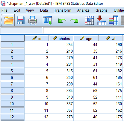
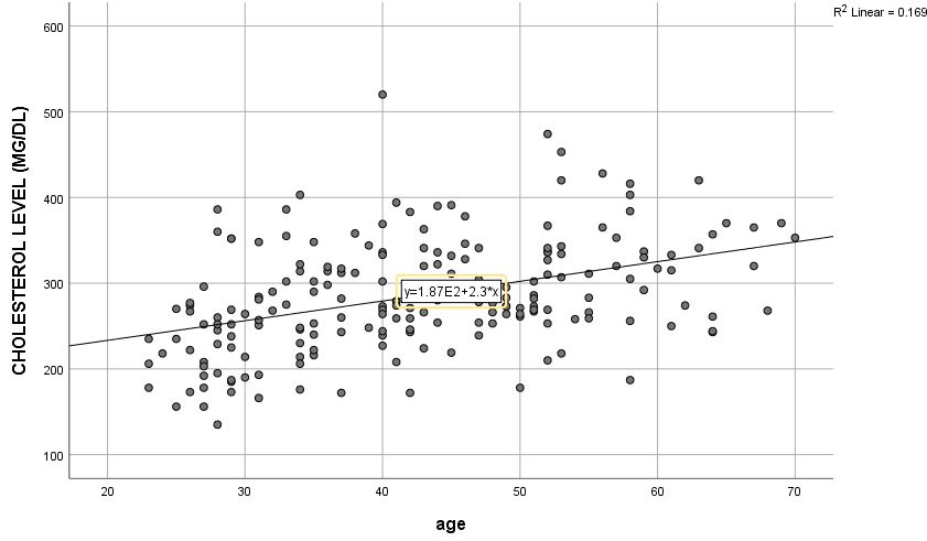
Suppose we have the set of scores shown at right in SPSS (e.g., chapman_1.sav). The correlation between cholesterol and age is $r = .411$ , a moderate value. A scatterplot of the data is shown below. Mostly the relation is linear.

Set of scores in SPSS

Screenshot of SPSS data

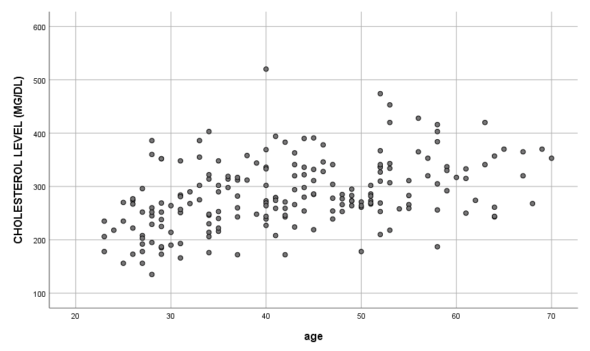
As mentioned earlier, correlation tells us about the strength and direction of the linear relationship between two quantitative variables. Regression gives a numerical description of how both variables vary together and allows us to make predictions based on that numerical description.

1. Inspecting the scatterplot

The scatterplot will show us a few things. Here’s what to look for:

(1) Does the relation look fairly linear?

(2) Are there any unusual points?

(3) How close to the line do most points fall?

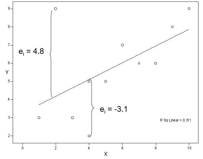
Let us now simplify the above plot to explain an unusual point better. One thing you should have noticed is that one point is far from the line and the other points.

Example scatterplot

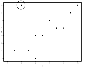
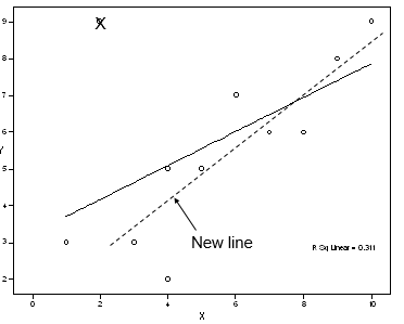
In this data, the relationship is fairly linear (aside from the one point), so we are happy about that. Let us see what happens when that point is removed. Let us compare two regression lines:

Graph that compares two regression lines

Old values: $r=.56$ $R^2$ =.31 $MSE = 2.11 = 3.247 + .46 X$ , where MSE is mean squared errors, and

New values: $r=.89$ $R^2$ =.79 $MSE = 1.36 = 1.352 + .71 X$

When the odd point is removed, the slope of the line increases, the $r$ and $R^2$ go up, and MSE drops. The new line has a better fit. Therefore, the inclusion of a point far away from the bulk of the data makes

the $r$ value drop and
the line become flatter. Flat lines mean little to no relationship between $X$ and $Y$ .

Also, we see that the value of $R^2$ shown on the plot (“R Sq Linear”) is much lower.

Points that appear very different from the rest are called “outliers”. We have both visual and statistical ways of identifying outliers. We will learn about the statistical ones in more detail later on, but for now, we can at least look at the plot and look for unusual points. The point we removed was unusual looking and may have been an “outlier”.

In this data, it was a point where the $Y$ was much higher than we would expect, given the $X$ score. Of course, we would want to examine the nature of the data for that case to assess whether there was an explanation for why the point was so unusual.

Caution: Do not just remove points without exploring why they may be unusual!

A point may be an outlier in this simple (one-predictor) model, but it may not look unusual if more variables are added to the model. Therefore, we need to be aware of possible outliers, but we should not permanently delete cases without a good reason until we have explored all models for the data.

2. Missing Data Analysis

Conduct missing-data and case analysis. We’ll check for missing subjects and missing values, and later examine individual cases as possible outliers or influential cases.

Part of what we need to do here is to find out whether cases are totally missing, or are missing some values on the outcome or predictor(s). In particular, if some cases are missing values for $X$ , we want to see if cases missing values on $X$ appear different from the cases with values for that $X$ .

It is difficult to analyze whether cases are missing at random or in some pattern, especially if we have no data for the cases. If we have some data for all subjects we can compare scores of those with complete data to those with some data missing.

However, even if our missing cases have no data at all, sometimes we have data on the population we are sampling and can make a judgment that way. Missing data analysis is another world of statistics, so we can skip it for this moment.

3. Case Analysis

We have already used a plot to see if our data seem unusual in any way. However, there are also statistical ways to analyze all of our cases to see if any cases seem unusual or have more influence on the regression than others.

Typically we will examine the cases in the context of a specific model. We can compute residuals and standardized residuals. Then, what are residuals?

Residuals are the differences between the observed $Y$ and the predicted $Y$ (by the model).

Observed $Y$

$Y_i = b_0 + b_1X_i + e_i$

Predicted regression model or estimated regression equation

$\hat{Y}_i = b_0 +b_1X_i$

$Y_i = \hat{Y}_i + e_i$

Subtract $\hat{Y}$ from $Y$ :

$e_i = Y_i - \hat{Y}_i$

Here $e_i$ is a residual.

Several kinds of residuals are defined. I will talk about raw residuals and standardized residuals.

First, raw residuals are simply distances from each point to the line:

$e_i = Y_i - \hat{Y}_i$

These are easy to interpret because they are in the $Y$ scale. For instance, if we are predicting GPAs on a 4.0 scale (0 to 4) and a case has a residual of 2, we know that is a large residual. For example, we may have predicted a GPA of 2.0 but the person had a 4.0 (or vice versa if the $e_i = -2$ ). The unusual case has a residual of nearly 5 points. The next largest residual is just about 3 points and most others are much smaller.

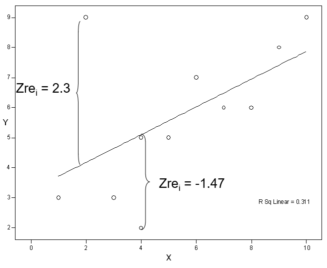
Graph displaying regression line and residuals

Second, standardized residuals are as follows:

$Zres_i = \frac{(Y_i - \hat{Y}_i)}{\sqrt{MSE}}$

Standardized residuals show the distance of a point from the line, relative to the spread of all residuals. If most points fit close to the line to predict GPA, then a point with a residual of 0.2 may be large.

We compute standardized residuals by dividing by their SD (SEE or RMSE = root MSE), so the standardized residuals have a variance or SD of about 1 (SPSS calls these ZRE_n: ZRE_1, ZRE_2, etc.). Here, SEE means standard error of estimate.

Typically we look for ZREs larger than 2 because these are 2 (or more) SDs away from zero. Again the unusual point has a large standardized residual of over 2 SDs. The next largest standardized residual is under 1.5 SDs and no others are above one SD.

Graph with ZREs

We will also see how to use residuals in the consideration of our assumptions – several of our assumptions are about the residuals from the regression line. If these assumptions are not satisfied, we must not run a regression analysis.

4. Checking Assumptions

We will do some analyses of residuals, and (for multiple regression) look for multicollinearity. This section will be later explained in detail.

II. Simple Regression in SPSS

Let us go back to chapman_1.sav that we had seen earlier.

Set of scores in SPSS

Screenshot of SPSS data

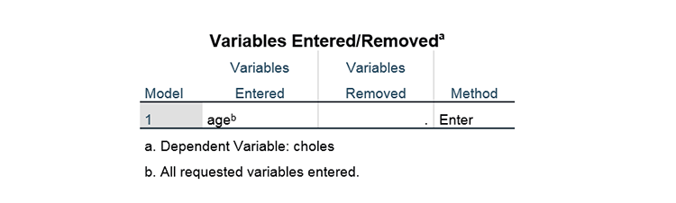
Here is SPSS output for the simple regression analysis.

The following part just tells us what $X$ we are using (i.e., age)

Table showing the experiment variables

Here we see the $r, R^2$ and adjusted $R^2$ for the data as well as the SEE.

Chart with model summary of experiment

$r = .411$

$r^2 = R^2= .169$

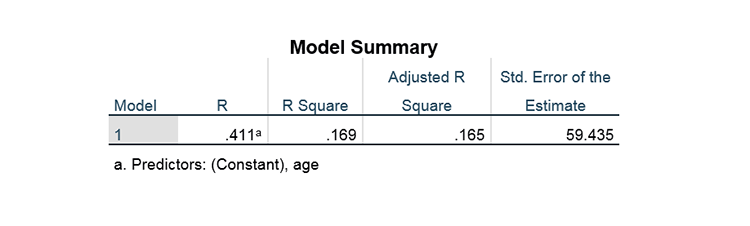
The correlation r is the correlation between $X$ and $Y$ . However, it is also the correlation between $Y$ and $\hat{Y}$ . Therefore r is telling us about how close the predicted values are to the observed values of $Y$ . Similarly $r^2$ or $R^2$ is the square of that value, r. Clearly, we want r to be big and also we want $R^2$ to be big.

When we have several $X$ , then $R^2$ will be the correlation between the $Y$ and predicted values that are based on all of the $X$ – so it is a measure that captures more than the set of individual $r_{xy}s$ for the $X$ in our model. $R^2$ is called the coefficient of determination.

We can interpret $R^2$ as the proportion of variance in $Y$ that is explained (= SSR/SST, where SSR is shorthand for the “Sum of Squares of Regression” and SST is shorthand for the “Sum of Squares of Total” ). In other words, $R^2$ is about how well all of the model with the independent variables is working to predict the dependent variable, therefore, we would like $R^2$ to be close to 1. Here, with $R^2 =.31$ we have explained about a third of the variation in $Y$ scores with this $X$ .

Namely, understanding the strength of independent variables (IVs) in predicting the dependent variable (DV) is via $R^2$ the coefficient of determination.

$R^2$ = SSR/SST = SSR/(SSR+SSE)
$R^2$ is the proportion of the variation in the DV that can be “explained” by the IVs.
The maximum value of $R^2$ is 1 (minimum is 0; no negative values).
SST: Total sum of squared deviations from the mean (i.e., Total variation in Y).
SSR: Sum of squared deviations from the $\hat{Y}$ and Ybar (i.e., Explained variation in Y).
SSE: Sum of squared deviation from Y and Ybar (i.e., Unexplained variation in Y).

[Exercise 2]

$R^2$ is about how well all of the IVs are working together to predict the DV. With an $R^2$ of .40, this means that 40% of the variation in DV (40% of the DV’s predictability) is explained by all the variables in the model. To understand what other unknown factors might help predict the DV, the researcher would consider what other variables to add to the model.

With an $R^2$ of .40, what percent (%) of the variation in DV is unexplained by all the variables in the model?

With an $R^2$ of .40, can you evaluate if the model predicts the DV well (Refer to Cohen’s rules of thumb below)?

We will learn more about the following table later, but for now, we use it to find the MSE (see the red circle below).

Table with ANOVA data

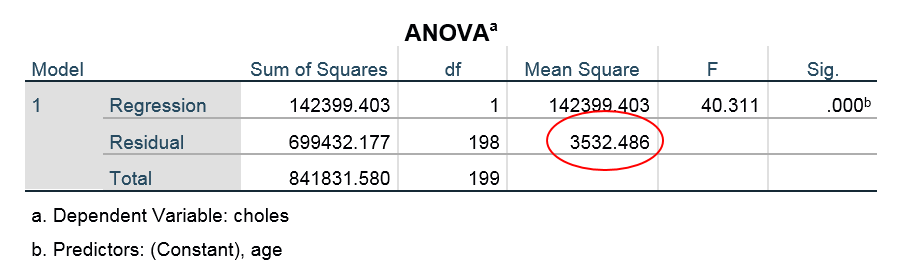
MSE = 3542.486 = $(59.435)^2$

SEE = 59.435

The MSE (see the ANOVA table) is the “Mean Squared Error” – actually this is the name for the variance of the $e_i$ values around the line. The closer the values are to the line, the smaller MSE will be. It is good for MSE to be small.

We can compare MSE to the variance of $Y$ . Here the variance of $Y$ is 4230.31, so our MSE of 3542.486 is a decent amount lower than ${S_Y}^2$ .

The SEE is just the SD of the $e_is$ , or $\sqrt{MSE}$ . Therefore, here SEE = 59.435 and can be compared to $S_Y$ , which is 65.041. This is telling us the same info as MSE, but SEE is in the score metric (not the squared metric). You can guess – SEE should also be small.

The following table contains the slope $(b_1)$ and Y-intercept $(b_0)$ as well as t-test of their values.

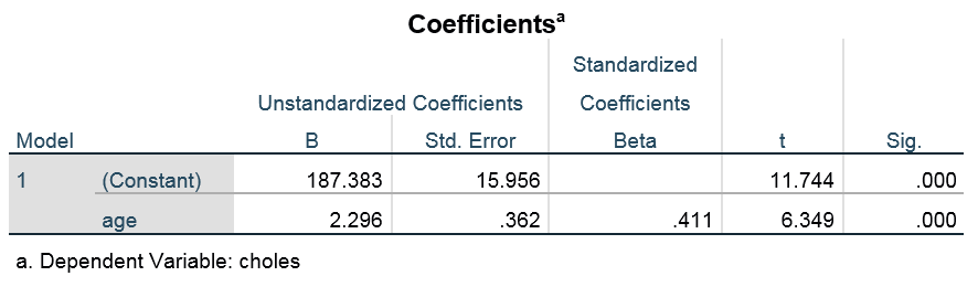
Table showing the coefficients of analysis

Scatterplot with estimated regression model

Based on the above table, an estimated regression model is written. We can call it a regression equation or regression line: $\hat{Y} = b_0 +b_1X$ , where $\hat{Y}$ is the expected value for the dependent variable.

As shown in the above scatterplot, SPSS computed it as

$\hat{Y} = 187.383 + 2.296 X$ , where $X$ is an independent variable, which is age, and $Y$ is cholesterol level.

Let us interpret Y-intercept $(b_0)$ from the above table. Here is a generic regression equation: $\hat{Y} = b_0 + b_1X$ .

$b_0$ is called the Y-intercept.
$b_0$ is the expected value of $Y$ when $X = 0$ .
This value is only meaningful when $X$ can have a realistic value of zero.

Expected cholesterol level $= b_0 +b_1 \ast age$

Plug the estimated value that the Coefficients table has in the equation (i.e., 187.383):

Table showing the coefficients of analysis Expected cholesterol level = 187.383 + 2.296*age

$b_0$ tells us that the expected cholesterol for patients at age 0 is 187.383.
First, what do you think of age 0? The average mean cholesterol level at age 0 is actually 70 (American Committee of Pediatric Biochemistry, 2019).
Second, the approximate value 187 on the Y-intercept is telling us that the patients’ cholesterol level would be 187 on average when age is 0. Therefore, for this case, treat this Y-intercept as one point on the regression line, but not one that is very relevant.

Now, let us interpret regression coefficient or slope $(b_1)$ from the above table. Here is a generic regression equation: $\hat{Y} = b_0 + b_1X$ .

$b_1$ is called the regression coefficient.
$b_1$ is the expected change/difference in $Y$ for a one-unit increase in $X$ .
Direction: Look at sign in front of $b_1$ .
Strength: The higher the value of $b_1$ , the more $Y$ responds to changes in $X$ .

Expected cholesterol level $= b_0 +b_1 \ast age$

Plug the estimated value that the Coefficients table has in the equation (i.e., 2.296):

Expected cholesterol level = 187.383 + 2.296*age

As the age of a patient increases by 1 (say, from 21 to 22), their cholesterol level increases by 2.296.
For each one-unit increase in age, patients’ cholesterol level increases by 2.296.

III. Standardized Slopes and Regression Model Tests

Earlier, we estimated the regression model. Here we get the values of $b_0$ and $b_1$ plus other indices we saw earlier (MSE, SEE), and also standardized slopes.

1. The F-Test for the Overall Model

We test the overall relationship using the F test. We learn how to test whether the model as a whole (the set of $Xs$ taken together) explains variation in $Y$ (the omnibus test = Overall test). If the overall relationship is significant, then, continue with the description of the effects of individual $Xs$ .

For the test of significance of the overall relationship – a test of $H_0: \rho^2 = 0$ or technically of

$H_0 = {\rho^2}_{Y\hat{Y}} = 0$

that is, a test of whether the outcome and predicted values are related. While in practice we test the overall model quality (i.e., F-test) before testing individual slopes. When we do the F test we want it to be large. We make the test as F = MSR/MSE. Also, F = SSR/MSE when we have one $X$ . We want SSR or MSR to be large, and MSE to be small. Both of those lead to a large F test.

So how do we do the F test? Let us use our chapman_1.sav data and compute

F = MSR/MSE = SSR/MSE = 142399.403/3532.486 = 40.311

Table with F test results

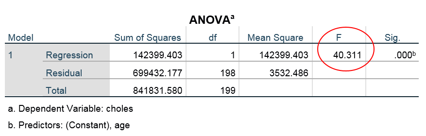
Then use the F table with the right df. In our original example, we have F(1,198). The F table in most statistics books shows that the critical value for the .05 test is 2.705. Our F is above the critical value, therefore, we reject $H_0$ . Also the printed $p =.000 < .05$ which gives the same decision.

Now, how do we interpret the F test? For our champan_1.sav data we reject $H_0$ , which we said was either:

$H_0: {\rho^2}_{Y\hat{Y}} = 0$ (or $H_0: \beta_1 = 0$ because this is a simple regression model)

therefore,

$H_0: {\rho^2}_{choles.\hat{choles.}} = 0$ (or $H_0: \beta_{age} = 0$ )

The value F = 40.311 would occur less than 5% of the time if either of these $H_0$ was true, and that is too unusual. So we decide probably these $H_0$ is not reasonable. In other words, our $X$ probably predicts $Y$ very well, so we decide $X$ has a nonzero slope $(i.e., \beta_1 \neq 0)$ thus predicts $Y$ , or the predicted $Y$ values relate to the actual $Ys: {\rho^2}_{Y\hat{Y}} \neq 0$ .

2. The T-Test for the Individual Slope Tests

We have the test of whether a slope is zero. For the test of significance of the individual slope – a test of $H_0: \beta_1 = 0$ is conducted. So far we have only one $X$ , so the test of $\beta_1 = 0$ (the t-test) will give the same decision as to the overall F test. Of course, the individual slope tests in multiple regression model are different from the overall F test.

We want to test whether the relationships that we see in the sample exist in the population. Many students often think that the job of researchers is to prove a hypothesis is true, but very often, they do the reverse: They set out to disprove a hypothesis, which is called a “null hypothesis”. Whether we reject the null hypothesis or not is usually decided with a 5 percent chance of being right. Namely, if we find that the odds of observing the data is less than 5 percent, then we could reject it.

A statistical hypothesis testing does not determine whether the null hypothesis or an alternative hypothesis is correct. This is a matter that can be answered only by knowing the true parameter, $\mu$ . We do not know the true value $\mu$ because inferential statistics are based on the results of examining only the sample, not the entire population.

The hypothesis test is only to find out whether the alternative hypothesis can be said to be correct when looking only at the sample results. The hypothesis test is not to analyze whether the null hypothesis can be said to be right. The null hypothesis is only an auxiliary hypothesis used to find out whether the alternative hypothesis can be judged correct.

Note your estimate of the population parameter may not be so good if your sampling design is not good. This issue is different from statistical analysis (You will learn about the sampling strategies in PUAD629). Researchers can develop the null hypothesis (i.e., $H_0$ ), which means that we believe that there is no relationship between $X$ and $Y$ . By virtue of you decide to conduct the study, you will always have a research (or alternative) hypothesis, which means that we believe that there is a relationship between the $X$ and the $Y$ .

Before we examine any tests, we will stop to consider how to decide if a slope is important. The importance here is independent of statistical significance – this relates to practical importance and to what is known about the outcome in the literature or in terms of theories. Also, we draw on conventional “rules of thumb.”

You may do this when comparing two different models (e.g., for two different $X$ variables), and in multiple regression, we will eventually want to choose among the predictors in one model to identify the most important $X$ (i.e., compare the magnitudes of $X$ s).

To do this we use the standardized regression equation. The slope $b_1$ depends on the scale of the $X$ variable as well as that of $Y$ . Therefore, if we want to compare slopes, we need to be sure they represent variables on the same scale. Unless two $X$ s have the same scale, we cannot compare their slopes.

Therefore, we need to equate the scales of the $X$ s. Note that, with the same logic, we would not able to compare the magnitudes of weight and height variables in raw scales because they use different scales, but once we standardize them, we can compare the magnitudes of these on $Y$ because standardized variables can be compared each other.

In sum, once we see whether or not the regression coefficients (i.e., unstandardized coefficient) are statistically significant, then we would like to see standardized coefficients because we want to compare the magnitudes of the significant variables on the $Y$ outcome. Here, the standardized coefficients are called beta-weights.

The beta-weights are about how well independent variables are pulling their weight to predict the dependent variables. Beta-weight is the average amount by which the dependent variable (DV) increases when the independent variable (IV) increases one standard deviation, controlling for all other IVs (held constant).

Think of multiple regression that has multiple $X$ s. We want to compare the magnitudes of $X$ s and to choose which one is the most important on $Y$ . We use beta-weight for it because it is scale-free.

We interpret beta-weight as follows: When $X$ (i.e., IV) changes (either increases or decreases) by one SD, the y-hat (i.e., estimated DV) changes by beta-weight SD, holding the other variables in the model constant.

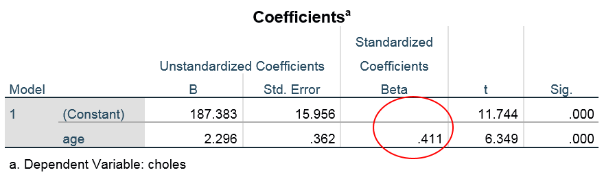Table with beta-weight circled in red We say the standardized slopes ( ${b\ast}_1$ ) is “the predicted number of standard deviations of change in $Y$ , for one-standard-deviation unit increase in $X.$ ” So if ${b\ast}_1 = .411$ we predict that $Y$ will increase by .411 of a SD, when $X$ increases one SD.

In contrast, regression coefficients are expressed in the units of measurement of Y-hat (estimated DV), and the units may not be comparable (e.g., age and blood pressure predict cholesterol but how can you compare the strengths between age and blood pressure because they have different units?). To make the scales comparable we compute a new score:

$Z(X_i) = \frac{(X_i - \overline{Y})}{S_X}$

where we subtract from each $X_i$ the mean and divide by the SD of $X$ . Recall that Z scores always have mean 0 and variance 1.

If we do this for all the $Xs$ (and $Ys$ ) the slopes computed based on those new Z scores will be comparable.

For single-predictor models this gives us a very simple equation:

$Z(Y_i) = {b\ast}_1 Z(X_i) + {e\ast}_i$

where ${b\ast}_1$ is the so-called “beta weight”. Note the intercept is 0 because both $Z(X)$ and $Z(Y)$ have means of 0.

We might also write the formula for the standardized regression line. As before we need to put a hat over the outcome to show it represents a predicted value.

$\hat{Z(Y_i)} = {b\ast}_1 Z(X_i)$

where $\hat{Z(Y_i)}$ = The predicted standardized score on $Y_i$ for case $i$ .

${b\ast}_1$ = the “beta weight” or “standardized coefficient”, the number of standard deviations of change predicted in $Y$ for one standard-deviation increase in $X$ .

$Z(X_i)$ = The standardized score on $X_i$ for case $i$ .

One last thing is true of beta weights in one-predictor regressions. That is, the standardized regression slope is equal to the correlation of $X$ with $Y$ in simple regression model. Therefore, ${b\ast}_1 = r_{XY}$ for the equation $Z(Y_i) = {b\ast}_1 Z(X_i) + {e\ast}_i$ . However, a standardized coefficient is not equal to the correlation between $X$ and $Y$ when we get to the multiple regression context.

Meanwhile, for bivariate (one-predictor) regression we can use rules of thumb for correlations to help interpret the sizes of the beta weights. Jacob Cohen (1988) provided a set of values that have been used to represent sizes of correlations, mean differences, and many other statistics (the so-called “Cohen’s rules of thumb”). These came from evaluations of the power of tests – but they have been widely used in social sciences in other situations.

For correlations, beta weights with only one $X$ , and $r^2$ the values are

	r or b*	r²
small	.10	.01
medium	.30	.09
large	.50	.25

Generally, we evaluate if a slope or a model predicts the DV well, according to Cohen’s rules of thumb.

[Exercise 3]

Read Zimmer’s article (2017), Why We Can’t Rule Out Bigfoot. Discuss how the null hypothesis can keep the hairy hominid alive in terms of falsifiability.

[Exercise 4]

Fill in the blank: We learned that the standardized slopes ( ${b\ast}_1$ ) is “the predicted number of standard deviations of change in $Y$ , for one-standard-deviation unit increase in $X.$ ” So if ${b\ast}_1 = .75$ we predict that $Y$ will increase by ( ) of a SD, when $X$ increases one SD.

Sources: Modified from the class notes of Salih Binici (2012) and Russell G. Almond (2012).

License

Icon for the Creative Commons Attribution-NonCommercial-ShareAlike 4.0 International License

Analytic Techniques for Public Management and Policy Copyright © 2021 by Jiwon N. Speers is licensed under a Creative Commons Attribution-NonCommercial-ShareAlike 4.0 International License, except where otherwise noted.