Chapter 4. Multiple Regression
So far we have worked with models for explaining outcomes when the outcome is continuous and there is only one continuous predictor. Now we will turn to multiple regression analysis, where we will be examining the roles of several predictors. There are many similarities between simple regression and multiple regression.
Unlike a simple regression that looks at the relationship between one independent variable (IV) and one dependent variable (DV), if we want to assess all IVs at one time the different associations that the DV has with multiple IVs, we can see that relationship better with a multiple regression. It helps us isolate the effects of IVs by controlling for the other variables.
I. Multiple Regression Models
In multiple regression, we are modeling variation in  via a model where
Outcome = Continuous Predictors + Error
or more specifically, the multiple regression population model for scores is

for case or person  with outcome
  (a continuous variable) and predictors
  through
  . The
. The  are still assumed to be independent and normally distributed with mean 0 and variance
  , as was true in simple regression. The error term () is defined as the difference between actual values and predicted values
  , which is generally called “residual”).
  is the intercept (value of when all
  equal 0) in the population,
  is the slope for predictor
  in the population, where the slope is the predicted change in for one unit increase in , holding all other X constant.
The regression estimated, fitted, or sample model is
 (the line)
where  is the score for case or person on outcome , and is the predicted score,
  , is the intercept (the predicted value of when all equal 0) in the sample,
  is the estimated slope for predictor , where the slope is the predicted change in for one unit increase in , holding all other X constant, and is the residual for person . If we write the model in terms of
  there is no term.
The underlined phrase is “holding all other constant.” This is how we specify that we are statistically controlling for the influence of other than the one whose slope we are interpreting. By including additional in the model, it is as if we were equating the cases whose scores we are analyzing on the added .
II. Adding Independent Variables
Suppose we are examining the role of CEO salary as a predictor of CEO performance.
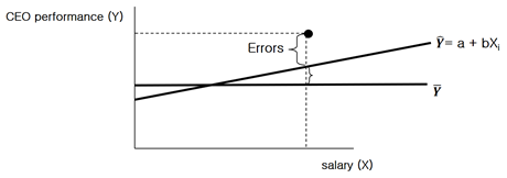
The errors are larger than the value predicted by the estimated regression line according to the above graph. Therefore, by putting another , say organizational ownership, into the regression model, we aim to decrease the sizes of the errors and it is also as if we have equated organizations on their ownerships. Then the slope of the original shows how much CEO salary affects CEO performance for the organizations with the same types of ownership (i.e., holding ownership constant).
When we have that are quite independent of each other, then adding an may not change the slope of the original at all. However, to the extent the overlap (are related to each other), we may see either bigger or smaller slopes for the original when a new is added. In either case, we hope that the added explain more variation in that just one alone. If they do, it will reduce the sizes of residuals (and thus reduce MSE), and therefore give us more powerful tests of the slopes in our model. Also adding should increase  , which is one of our indices of model quality.
Meanwhile, a control variable is defined as a variable held constant to assess or clarify the relationship between other variables. It is a variable that influences the DV, but not of a researcher’s immediate interests unlike the IV (i.e., CEO salary). For instance, let us say, the researcher’s main interest is whether or not the CEO salary (IV) is positively associated with his or her performance (DV). By controlling for organizational ownership (i.e., control variable), we are seeking to understand the CEO performance (DV) predicted by the CEO salary (IV) with the same types of organizational ownership (control variable). Here, the organizational ownership includes for-profit organizations, government organizations, and nonprofit organizations. Are CEO performance different due to the CEO’s salaries?
III. Assumptions in Multiple Regression
Aside from assuming independence and normality and equal-variances of residuals as noted above, another assumption that we are again making is that our model is properly specified. That is, we need to assume that (1) we have all the important X in the regression model, and (2) we have no irrelevant X in the model. These two assumptions, together with the assumption of linearity of the X-Y relationships, represent our assumptions about “model specification.”
3-1. Model Specification
With multiple regression, we will have a way to check these two assumptions. We will therefore learn how to assess “model specification.” When we say we have a properly specified model we are saying that we have the “right” or “correct” model — all the variables in the model (and no others) have linear relationships to in the population. Having a properly specified model is important because it has implications for our estimates.
One new issue is that multiple regression models assume that the predictors are independent of each other, but sometimes they are not. In the ANOVA case (where the predictors are categorical) we can be sure predictors are independent (not “confounded”) by making sure the group sizes are equal (or proportional). This is most strictly controlled in experimental designs where subjects are often randomly assigned to groups in equal numbers.
However, we do not typically assign people to have particular values of the in regression analyses. Therefore, we will need methods for assessing whether our are interrelated or “collinear.” The problem of having interrelated is called multicollinearity. In the next section, we will learn to assess whether multicollinearity is a problem for our models.
3-2. Multicollinearity
Multiple regression analysis uses several independent variables, and if these independent variables have strong correlations, the results of regression analysis are significantly less accurate. For example, suppose that two independent variables, and  are selected, and the observed data (
 ) are
) are
(1, 2, 11), (3, 6, 25), (-2, -4, -10), (2, 4, 18)
According to this data,  is always twice
  . Therefore, it can be seen that it has a relationship of
  . Let’s say that from the above data, for example, we estimated the regression equation
  . Then, due to the relationship
  can also be said to be an appropriate regression equation. Therefore, it is not known which of these two equations is an appropriate regression equation because it is impossible to distinguish whether the change of the dependent variable is due to the independent variable or . Therefore, in this case it becomes impossible to estimate the regression equation.
When multicollinearity is a problem, an example of the most effective countermeasure is to combine the variables into one. For instance, let us say is the number of men and is the number of women. At this time, if the number of men and the number of women changes approximately proportionally, strong multicollinearity occurs between the two variables.
In this case, this problem can be eliminated by introducing only one variable, the total population, rather than introducing these two variables separately. However, if it is theoretically desirable to consider both introduced variables, removing one of them can significantly reduce the explanatory power of the model.
In most multiple regression analyses, some multicollinearity usually exists. In particular, when the number of independent variables is plural, the possibility of multicollinearity is high. Even in the case of such high multicollinearity, multiple regression analysis is not at all meaningless.
When multicollinearity becomes a problem in regression analysis, it is necessary to be careful in interpreting the analysis results. In other words, there are many problems in determining the value of the coefficient of each variable (i.e., the significance of individual variables is unclear), but the value of the dependent variable produced by combining all of these variables provides a sort of accurate predictive value (i.e. the overall model combining individual variables can be significant).
Of course, in this case, if the values of the independent variables to be input are data found in actual reality, it means that there is a correlation between the independent variables through the values in this data. In addition, meaningful prediction of the value of the dependent variable is possible by inputting the data of these independent variables.
However, if you create and use artifacts that do not show correlation between independent variables (i.e., if you estimate the dependent variable for the values of independent variables that do not have correlation), the estimate will be difficult to trust and you will get meaningless results.
IV. Goodness of Model
Many of the analyses for multiple regression have tests and procedures similar to those we have learned already. For instance, we will see MSE and SEE, we’ll use F tests for gauging significance of the whole model, and we’ll have to assess whether assumptions about our residuals are appropriate using plots of the residuals. We will use the “variance explained” measure to assess whether the set of we have chosen is helping us to understand variation in the outcome. We will also have tests of the individual predictors that will be t tests.
How do we begin using multiple regression? First of course we need to have some idea of what predictors might reasonably be used to explain why scores vary. A starting point is what theory or prior research suggest might be good variables to use as through .
Also we will learn how to interpret the values of the slopes,  through
  , as well as how to decide which predictors are not useful, which predictor (of the useful ones) is most important, and how much we have explained about with the set of variables we’ve chosen.
Meanwhile, we will see that it is possible to examine categorical predictors using regression, but when there are multi-category variables it is very tedious and the ANOVA framework is more sensible and easier to use.
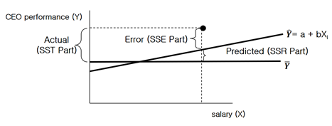
As in simple regression, in multiple regression, SST (i.e., the total variable of the dependent variable) is divided into two parts as follows:
![\Sigma{(Y_i - \bar{Y})}^2 = \Sigma{[(a + bx_i) - \bar{Y}]}^2 + \Sigma{[Y_i - (a + bx_i)]}^2](https://ubalt.pressbooks.pub/app/uploads/quicklatex/quicklatex.com-a5a15ce575ca01c1dac1cf0750b90963_l3.png "Rendered by QuickLaTeX.com")
Where SST = SSR + SSE
The left term is Sum of Squares Total (SST), which is total variation around the average of Y. The right term consists of SSR and SSE, which are variation explained by the regression line and variation not explained by the regression line, respectively. Also, the coefficient of determination, , is represented as

is the rate of the verified variation to the total variation. This effect size is widely used to assess the adequacy of regression analysis. However, in multiple regression analysis, when an independent variable is added, the coefficient of determination increases. Even when an independent variable that is thought to be completely independent of the dependent variable is added, there may be a slight correlation between observed data by chance, and in this case, the value of the increases by adding this new variable.
Therefore, statistical analysts who are inexperienced are likely to make an error in determining that this model is meaningful after increasing the value of the coefficient of determination by adding many meaningless independent variables. It is adjusted that was introduced to correct this error.
When one variable is added, the residuals continue to decrease, so the SSE value decreases, the ratio of the sum of residual squares to the total sum of squares (i.e.,  ) decreases; and increases. In this case, to prevent the error of increasing the value of the by introducing a meaningless independent variable randomly, adjusted is used and it is defined as follows:
Adjusted 
where  is the number of independent variables.
V. Dummy Variable
Even though we have multi-category variables (e.g., race group: Black, White, Hispanic and Asian), we can only use dichotomies (dummy variables) in multiple regression. Thus, we must learn to use dummy variables to represent multi-category factors.
First, a dummy variable is a dichotomy coded as a 0/1 variable. If ‘gender’ is the variable we may code a gender dummy variable where
 if subject is female (0 = reference group),
 if subject is male (1 = focal group).
Dummy variables can be used in multiple regression. When we use a dichotomy like in multiple regression, we get the typical estimated equation

 represents the predicted change in associated with 1 unit increase in
  . When one point change occurs in the scale of , a change of the amount would change in .
But when is a dummy variable () and only takes on two values (0 = female, 1 = male), a difference of one point can only occur when is equal to 1. When  , the subject is female, but when
  , the subject is male.
So, the slope for our bivariate regression where is a dummy variable equals the mean difference between the two represented groups – for this the slope is the difference between the means of males and females. Also we can see that
will equal  when
when  .
.
: Mean difference between male and female groups
: the intercept represents the mean of for the females (i.e., the mean for all cases with ).
It is easier to see this empirically by running descriptive statistics and a t test on two groups, and then running a regression using a dummy variable that represents the 2 groups as our .
We will see t test output for tchcomm with a variable that represents public vs private schools (“public”) as our predictor as well as a regression using that dummy variable.
The variable “public” has two levels: 1 for public schools, and 0 for all other schools (e.g., private)
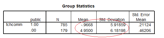
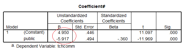
Coefficients table shows the slope equals the mean difference from the descriptive statistics and t output: -5.918= (-0.9668) – (4.95) (See Group Statistics and Coefficients)
The circle shows the value of the t test for the slope equals the two-sample t test. Also the intercept equals the mean of the reference group (= private schools):
The above results only hold exactly for a dummy variable coded 0 and 1.
If the dichotomy is coded with numbers that are not one unit apart (e.g., 1 and 2), then the slope will not equal the mean difference.
You can check this by running a regression using a dummy variable that represents the 2 groups with numbers other than 0 and 1. You will know that it is convenient that you assign 0 to a reference group and 1 to a focal group. What about a categorical variable that consists of three values?
Suppose now we have 3 groups (label, level), say, urban, suburban and rural schools. We have a variable g10urban
X = 1 for urban schools
X = 2 for suburban schools, and
X = 3 for rural schools
If we include g10urban in a regression, multiple regression will treat it as if it were a number, not a label. Is a suburban school ( ) “twice” as good as an urban one ()? So using in multiple regression as it is would be a mistake.
This is not something that we try to do. Note that SPSS [machine] does not stop you from using a categorical variable in regression, as if the  variable is a continuous numeric variable. Here is output using g10urban to predict tchcomm, which is wrong:
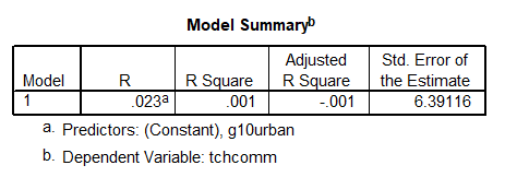
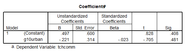
We use dummy (0/1) variables to differentiate these 3 groups (label); however, SPSS mistakenly takes the variable as a numeric variable. So we need to represent the 3 groups in some other way: Conversion of the number into dummy variables.
We will use (k-1) dummy variables to represent k groups.
Let  represent ‘Is the school urban?’(1 = Yes) and
  represent ‘Is the school suburban?’ (1 = Yes).
If we have one school from each group, their values of the original factor (g10urban) and the two dummy variables and would be
School Level chart forthcoming
Again here are the scores:
School Group chart forthcoming
We do not need a third variable ( ) that represents ‘Is the school rural?’ (1 = Yes).
The pair of values (, ) is different for each group of subjects so we can tell 3 groups apart using 2 dummy variables.
Also note, we interpret  as the difference between urban schools and all others, holding constant.

For all the urban schools,  and
and  , so
, so 
For the others,
if they are rural, (and  ) therefore
 if they are suburban, (and
  ) therefore
Because of the way we created and , we will never have a case where both and .
Suppose now that we use the variables and in multiple regression. In our estimated regression equation

or

the value of is the mean (or predicted score) for the rural schools, which is the predicted value of when the values of all the are zero.
In a case such as this we might actually be interested in testing whether  because represents the population mean of the rural schools.
With the intercept and two slopes we can compute all of the group means.
Our estimated regression equation will be
The slope represents predicted change in for 1 unit increase in , holding constant.
It is also the difference between the urban group mean and the mean for the reference group of rural schools.
The slope  represents predicted change in for 1 unit increase in , holding constant, and it is the mean difference between the suburban schools and the reference group of rural schools.
Specifically we can see that
 for rural schools
 for urban schools
 for suburban schools
None of our cases ever has

because no school can be in two locations.
The school means on tchcomm are
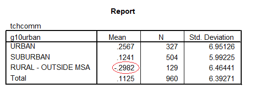
The regression is
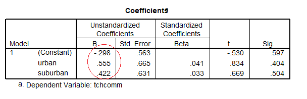
So b0 = -.298 the rural mean (these are circled)
b0 + b1 = -.298 + .555 = .257 the urban mean
b0 + b2 = -.298 + .422 = .124 the suburban mean
VI. Recode a categorical variable into dummy variables in SPSS
In the SPSS “variable view” we can find out that g10urban is coded with
- 1 = urban
- 2 = suburban
- 3 = rural.
In addition, there are several schools with missing values on this variable. We have learned that we need 2 dummy variables to represent these 3 groups. Let’s name these 2 dummy variables as “urban” and “suburban,” so that:
- Urban: if school type is urban, then coded as 1, otherwise, coded as 0
- Suburban: if school type is suburban, then coded as 1, otherwise, coded as 0
The following few images guide you on how to create “urban.” You need to do “suburban” by yourself with similar procedure.
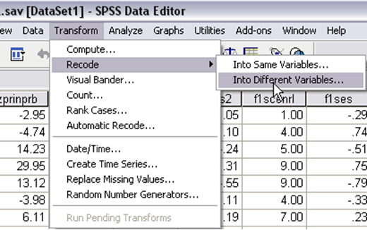
Step 1. To create dummy variable called “Urban,” go to SPSS > Transform > Recode > Into Different Variables…
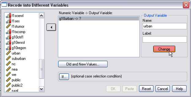
Step 2. Select your target variable “g10urban” > give a name to your dummy variable which is urban, > click “change” > click “Old and New Values,” it will pop up a new window, asking you to define the new and old values.
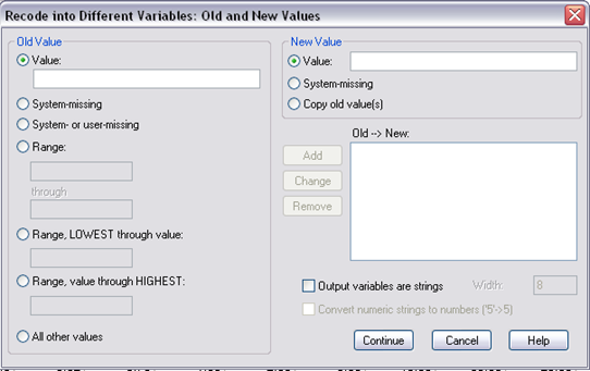
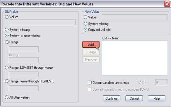
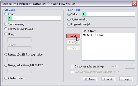
Step 3. This is the pop-up window, in here, you need to define old value and new value. First, select “system- or user-missing” on the left and “copy old values” on the right, then click “add.” Doing so is because there were several missing values in this variable.
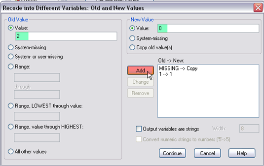
Step 4. Next, select “value” and enter 1 on the left, select “value” and enter 1 on the right, then click “add.” Doing so is to recode g10urban=1 (remember g10urban=1 is for urban school) as “urban=1.”
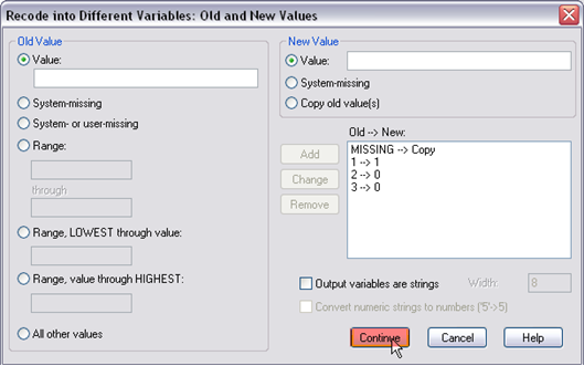
Step 5. Next, select “value” and enter 2 on the left, select “value” and enter 0 on the right, then click “add.” Doing so is to recode g10urban=2 (remember g10urban=2 is for suburban school) as “urban=0.”
Step 6. Next, select “value” and enter 3 on the left, select “value” and enter 0 on the right, then click “add.” Doing so is to recode g10urban=3 (remember g10urban=3 is for rural school) as “urban=0.” This is what the window looks like after you define values, then click “continue,” and “OK” in the main window.
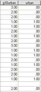
Step 7. Finally, go to the data view window, you should find there is a new variable called “urban.” As you will find now, g10urban=3 or 2 were recoded as urban=0, g10urban=3 were recoded as urban=0, and the original missing values are still coded as “missing.”
[Exercise 7]
Now you are asked to run a simple regression model with dummy variables converted from “g10urban.” In the simple regression model with dummy variables, there is no other predictors except the categorical one that you applied dummy codings for. Using the pull-down menu SPSS > Regression > Linear > Linear Regression… , locate tchcomm to “Dependent.” What variables are you going to move to “Independent(s)”?
VII. Detecting Interactions
Now that we have seen that we can use dummy variables in multiple regression to represent groups, we will tackle another idea.
Suppose we are examining a regression model with a dummy variable and we expect that relates to differently in our 2 groups. Say we are studying the prediction of the outcome of tchcomm scores for public and private schools, and we believe tchcomm relates differently to the predictor of principal leadership in the two school types.

We can say that there is an interaction ( ) of school type and principal leadership with respect to the teacher community outcome.
How can we tell if we need to be concerned about an interaction like this? One way is to let SPSS help us find it by using the scatter plot. Another is to examine the correlations or slopes.
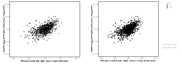
Pull down the Graph menu and make a scatterplot where is the variable (tchcomm) and is prinlead. Before you click “OK,” move the variable “public” into the “Set Markers by” box.
This forces SPSS to use different symbols for public and private schools and enables us to edit (double-click) the plot then use “Chart Options” to plot separate regressions for the school types.
On the left is the plot without markers – the relationship looks linear. Then we add the markers by public and plot two lines. The lines are not so different. The lines look parallel.
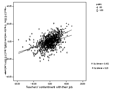
Here is a plot for tchhappy as the predictor.
When we add the markers by public and plot two lines they cross. These lines appear to have somewhat different slopes, so there may be an interaction.
In order to see an interaction, are you going to run two separate regression analyses for the groups involved (e.g., public and private schools)? No, don’t do it. There are drawbacks to this (i.e., Do not split the file and run a model with only the predictor variable in it, omitting the dummy variable).
- First, the sample size for the regressions will be much smaller because we will do two analyses, on two split data.
- Second, we will end up with separate slopes and need to do computations by hand to test whether the slopes differ by school type. With this approach we run separate regressions for the groups involved if we see a potential interaction. However, a more parsimonious solution would be to model the two slopes via an interaction in a single regression model. Also this approach gives us a test of the interaction (i.e., the difference between the slopes).
To do this we need to compute an interaction variable. Suppose is the “public” dummy variable and is tchhappy. Then we compute the product  . This new variable takes on values as follows:
 , if the school is private (0 = reference group), plug 0 to , then
  becomes 0,
, if the school is public (1 = focal group), plug 1 to , then becomes .
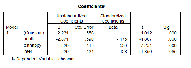
For the more elegant solution we run a regression that includes (the dummy variable), (the continuous predictor), and (the interaction) so our model is

- represents the public-private mean difference (or here intercept difference), controlling for and ,
 represents the slope of the predictor tchhappy, controlling for (school type differences) and (the interaction), and
- is the interaction, or the school-type difference in the tchhappy slopes, controlling for and .
Because is a dummy variable and also because takes on the value 0 for private schools, the two school types have different models that we can determine even without running SPSS to estimate the model. ( = School type dummy, = Covariate, )
For private schools, the value 0 is plugged for and ; those variables do not appear in the model for private schools. The private school model is

For the public schools, the variables are  and
and  . Thus the public school model is


From this output we can see that the private school estimated regression line is

Also we can compute the other model.
The intercept is:  and the slope
  .
.
Therefore, the public school model was


SPSS also then tells us whether the interaction is significant.
In this output we see that  does not have a significant slope. So even though the lines look a bit different, they are not quite different enough, so we do not need to keep the interaction variable in the model.
Sources: Modified from the class notes of Salih Binici (2012) and Russell G. Almond (2012).
