Part 1 of the lab will utilize data for the number of homicides in Baltimore between 2010 and 2019. All crime data is derived from The Baltimore Sun’s reporting of homicides in the city. The population estimates are derived from the U.S. Census and the American Community survey comes from the Bureau of Justice Statistics report. In this part of the lab, you will be computing the homicide rate for Baltimore.

Part 1: Homicides in Baltimore

Data Entry

1. Open up a new Excel worksheet. You will enter a new set of data into Excel in this lab.

a. I will refer to a cell by its name in Excel. For example, Cell B4 is in column B and row 4.

b. A range of cells selected together is defined by its “address,” which is the first cell and last cell in the rage of selected cells. So, if we select all the cells B4, B5, C4, and C5, the address would be “B4:C5” because it contains the cells from B4 to C5.

2. Click cell B4 to make it the active cell.

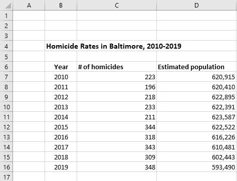
a. Type Homicide Rates in Baltimore, 2010–2019. Press Enter.

i. Note: The title does not fit in the cell B4 and spreads across several columns. If a label does not fit in a cell, it will display the remaining text in the next cell(s) as long as they are empty. Otherwise, the label is truncated or cut off.

b. Click cell B5 to make it the active cell and type Year.

c. Click cell C5 and type # of homicides.

d. Click cell D5 and type Estimated Population.

3. Notice that the labels truncated (or cut off). However, if you place the cursor on the cell, the full text appears in the formula bar. Don’t worry about the truncation for now; we will fix it later.

4. Enter the data from the table provided below into the worksheet in the appropriate cells of the table. The placement and formatting may not be exactly like the picture below—that is okay. We will format the table later.

a. Some of the population figures will be too large for the standard cell width, so they will be displayed with a series of number signs: ####. The data are there; it’s just that the column is too small to display all of the numbers.

5. You may notice in the picture that the title is separated from the data. To do this, we will insert a row.

a. To insert a row, move the cursor to row number 5. At the beginning of the row is the shaded box with the row number 5 inside. Click on the shaded box 5 and the whole row will become highlighted. Right click on the row and select Insert to add in a new row.

6. Now we will format the cells so that they display the data better. First, center the Year label and the data in those cells.

a. Select the range beginning with the Year label down to the cell containing the last year of 2019 (cell range B6:B16). Under the Home menu at the top of the page, with the range highlighted, select Center from the Alignment group in order to center the text in this group.

7. Now we want to make the titles for the homicides and population columns more readable and we want to see all of the population figures displayed in the cells.

a. First, we will extend the width of these two columns. To do this, select the range of cells from C6:D16. Select Format from the Cells group at the top of the page, and then select Column Width. A box appears with the default width. Press the delete key to clear the box and type 22 to make it the new column width, then select OK.

8. Next, we want to wrap the text of the labels for the homicide and population columns.

a. To do this, click on the cell which has the label for the # of homicides column. Select the Wrap Text button from the Alignment group at the top of the page. Do the same for the label for Estimated Population.

9. Now, make a new column for our calculation of the Homicide Rates.

a. In cell E6, type in Homicide Rate and with the cell active, select Wrap Text. Save your workbook again, and now we’ll move onto something slightly more complicated.

Entering Formulas

10. Formulas are used to perform numeric calculations such as adding, multiplying, and averaging. Formulas always begin with a prefix of an equal sign (=), and use arithmetic operations (+, -, *, /) to perform calculations: (+) performs addition, (-) performs subtraction, (*) performs multiplication, and (/) performs division.

a. Formulas can contain more than one arithmetic operator and allow for the use of parentheses. In these circumstances, Excel decides which operations to perform first. Multiplication and division are done first, based on a left-to-right flow. Addition and subtraction are performed after that.

11. Formulas often contain cell addresses and ranges. Using a cell address or range name in a formula is called cell referencing. Use cell references to keep your worksheet up-to-date and accurate. If you change a value in a cell, the formula containing that cell reference will automatically be recalculated using the new value.

12. Calculating Rates: Rates are one of the most common formulas in criminal justice. A rate is essentially the number of times something happens per X number of people in the population.

a. Example: 25 motor vehicle thefts per 100,000 people each year.

13. The formula for calculating rates is:

a. Note: this is for rates per 100,000 people, which we will be using in this lab. However, this can be changed to represent any other interval of people we want, like 1,000 or 100.

14. For the year 2010, how do you calculate the Homicide Rate?

homicides per people.

15. How would you construct the formula using cell referencing?

16. Now we want to have a rate for each year. Essentially, we want a fourth column of data which contains the rate for each year. This is our Homicide Rate column. Label cell E6 with this label and adjust the width as needed to make sure it can be visible.

a. Make E7 the active cell. In that cell, type: =(c7/d7)*100000

b. Then hit Enter.

c. Using cell referencing in formulas is convenient because instead of having to type a new formula for each additional year, Excel can now transfer the same formula down the rows for the same column, which saves you from writing a new formula for each year.

d. To use cell referencing in formulas, make E7 the active cell. Select Copy from the Clipboard group (the icon is right below the cut icon and looks like two overlapping pieces of paper). [Note: You can also 1) simultaneously hold down the CTRL and C buttons or 2) right click and select Copy].

e. Now select the range E8:E16. When the range is highlighted, select Paste from the Clipboard group.

f. The formulas for the rate for each year are now created, and the rates are displayed. Excel simply updated your original formula for each row, which saves you a lot of time and effort. Press ESC so that the cell you just copied is no longer active.

17. Let’s say we only want one decimal place for the rate.

a. To change the decimal place and round the numbers off, select the range E7:E17.

b. Under the Home category, in the Number group, find the button for decreasing the decimal place (called Decrease Decimal). Keep clicking on the button until only one decimal place is displayed. Save your work.

18. Your table should now look like this:

Using Excel Functions

19. Functions are predetermined worksheet formulas that enable you to do complex calculations easily without writing formulas. Functions begin with the prefix (=). We will use the Sum function to add up the total number of deaths for all the years.

20. Make cell B19 active. Type Total into the cell in order to label this row. Now, make cell C19 active so we can use our first Function.

a. In the top ribbon, select the Formulas tab. In that tab, position the cursor over the Auto-Sum button, the box with the capital Greek letter E ( ∑ ), and click/select it.

b. Auto-Sum sets up the sum function to add values in the cells above the cell pointer.

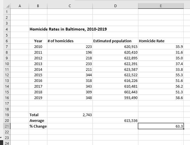
c. Here the formula =SUM (C7:C18) appears in the cell, which is the full column under the label. Verify this range and press Enter. The results now appear in the cell: 2,743 is our total number of homicides from 2010–2019.

21. Another function Excel provides is the averaging function, which would allow you, for example, to calculate the average population for all the years. Let’s try that.

a. Make cell B20 active and type Average into the cell to label this row.

b. Instead of typing in a formula to do an average, you can use the Function Wizard for fast and accurate calculation.

c. To use the Function Wizard, make the D20 cell active (we’ll be replicating something similar what we just did for Sum).

d. Now, we will want to calculate the average for this column. To do this, go back to the Auto Sum box but now click on the little arrow next to it. You will get a few options for formulas. Select Average.

e. Here the formula =AVERAGE(D7:D19) appears in the cell, which is the full column under the label. Verify this range and press Enter. The results now appear in the cell: 615,536 is our average estimated population per year.

22. We’re also interested in finding the percent change in the homicide rate from 2010 to 2019 (note that this is for the entire time frame, not from year to year). What is the formula for calculating the percent change from 2010 to 2019?

How would you construct the formula using the Excel cell reference method?

23. Fortunately, Excel can perform complex operations involving numerous steps; in this case, subtraction, multiplication, and division to calculate the percent change.

a. Click cell B21 to make it active and type % Change in order to label the row.

b. Select cell E21. Based on the percent change formula, we need to subtract the most recent date (2019, time 2) and the first date (2010, time 1) and then divide it from the first data point we have (2010, time 1). We also have to make sure to follow order of operations; if we do not use parentheses, Excel will give us a meaningless answer.

c. As such, we need to type in cell E21: =(E16-E7)/E7*100

d. Then hit enter. This calculates the percent change in the homicide rate from 2010 to 2019.

e. Here, this answer is 63.3%, thus we had a 63.3 % increase in homicide rate from 2010–2019.

24. The final results should look like the table below. Please check your work to make sure the numbers and equations are the same!